Building a 3D Pharmacophore Model from PDB Data: A Free Python Workflow

Build the pharmacophore from ligands that already bind the pocket. Overlay them, keep the shared features, and the distances between those features are the screening query. This note does that with biotite, MDAnalysis, scikit-learn, and RDKit. The example target is EGFR, UniProt P00533.
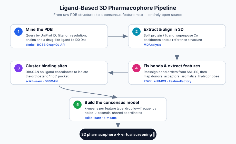
A 3D pharmacophore is the spatial pattern a binder has to present: hydrogen-bond donors and acceptors, aromatic rings, hydrophobic contacts, and the geometry between them. Ligands that occupy the same site tend to place the same features in the same place. Collect those complexes, put them in one frame, and keep the features the set agrees on.
1. Mining the Protein Data Bank
Ask the RCSB PDB through biotite and the GraphQL search API. The block below is the quality filter, joined with operator="and":
- UniProt accession, exact match (P00533),
- method X-RAY DIFFRACTION,
- combined resolution ≤ 3.0 Å,
- a chemical component with formula weight greater than 100, which drops ions, water, and most buffer molecules.
import requests
import biotite.database.rcsb as rcsb

UNIPROT_ID = "P00533"  # e.g. EGFR

# Build a composite query against the RCSB search API
query = rcsb.CompositeQuery(
    [
        rcsb.FieldQuery(
            "rcsb_polymer_entity_container_identifiers."
            "reference_sequence_identifiers.database_accession",
            exact_match=UNIPROT_ID,
        ),
        rcsb.FieldQuery("exptl.method", exact_match="X-RAY DIFFRACTION"),
        rcsb.FieldQuery(
            "rcsb_entry_info.resolution_combined", less_or_equal=3.0
        ),
        rcsb.FieldQuery(
            "chem_comp.formula_weight", greater=100  # drug-like ligand
        ),
    ],
    operator="and",
)

pdb_ids = rcsb.search(query)
print(f"{len(pdb_ids)} structures passed QC: {pdb_ids[:10]} ...")
rcsb.search returns the PDB IDs. The print line reports how many passed and shows the first ten. Coordinate download comes after this block.
2. Extraction and 3D alignment
Each crystal structure has its own frame, so the ligands cannot be compared until the proteins share one. MDAnalysis reads a high-resolution reference and each mobile PDB, superposes Cα atoms, and copies the ligand coordinates in that frame.
align.alignto uses select="name CA" and match_atoms=False. The ligand selection is not protein and not resname HOH. The overlay treats the pocket as rigid relative to the fold.
import MDAnalysis as mda
from MDAnalysis.analysis import align

ref = mda.Universe("reference.pdb")          # high-resolution template
aligned_ligands = []

for pdb_id in pdb_ids:
    mobile = mda.Universe(f"{pdb_id}.pdb")

    # superpose Cα backbones onto the reference
    align.alignto(
        mobile, ref,
        select="name CA",
        match_atoms=False,
    )

    # the ligand now sits in the reference frame
    ligand = mobile.select_atoms("not protein and not resname HOH")
    aligned_ligands.append(ligand.positions.copy())
After the loop, every copied ligand lives in the reference frame.
3. Spatial clustering with DBSCAN
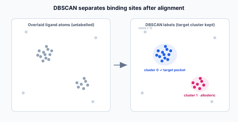
The query above accepts a ligand in any site. Orthosteric and allosteric binders both pass, and after the overlay they sit in different clouds.
DBSCAN finds those clouds from density. It takes clusters of any shape, marks sparse points as noise, and does not need the number of sites in advance. The settings here are eps=4.0 and min_samples=10. Label −1 is noise. np.bincount on the remaining labels keeps the densest cluster.
import numpy as np
from sklearn.cluster import DBSCAN

# pool every atom from every aligned ligand
all_coords = np.vstack(aligned_ligands)

db = DBSCAN(eps=4.0, min_samples=10).fit(all_coords)
labels = db.labels_

# keep the densest cluster - our target pocket
valid = labels[labels != -1]
target_label = np.bincount(valid).argmax()
pocket_mask = labels == target_label

print(f"Target pocket holds {pocket_mask.sum()} atoms "
      f"across {len(set(valid))} detected site(s)")
pocket_mask is an atom mask. The ligands that contribute atoms to that densest cluster are the ones carried into featurization. The print line also reports how many sites DBSCAN found.
4. Feature extraction and bond correction
PDB ligand records often store every bond as a single bond. An aromatic ring, a carbonyl, and a carboxylate then look the same, and every feature extracted from that file is wrong.
Take bond orders from the 2D SMILES in the PDB chemical component dictionary and copy them onto the 3D coordinates with AllChem.AssignBondOrdersFromTemplate, then Chem.SanitizeMol. rdFMCS is available when the template and the 3D atom set only partly overlap, via a maximum common substructure. This block runs the template assignment.
The feature factory is BaseFeatures.fdef. Each row is a family and a coordinate. The comment at the bottom of the block is the shape of one row: ('Donor', (12.3, 4.1, -2.0)).
from rdkit import Chem
from rdkit.Chem import AllChem
from rdkit.Chem import ChemicalFeatures
from rdkit import RDConfig
import os

# 1. fix bond orders using the 2D SMILES as a template
template = Chem.MolFromSmiles(ligand_smiles)          # correct chemistry
mol_3d   = Chem.MolFromPDBFile("ligand.pdb", removeHs=False)
mol      = AllChem.AssignBondOrdersFromTemplate(template, mol_3d)
Chem.SanitizeMol(mol)

# 2. map pharmacophoric features in 3D
fdef = os.path.join(RDConfig.RDDataDir, "BaseFeatures.fdef")
factory = ChemicalFeatures.BuildFeatureFactory(fdef)

features = []
conf = mol.GetConformer()
for f in factory.GetFeaturesForMol(mol):
    pos = f.GetPos()
    features.append((f.GetFamily(), (pos.x, pos.y, pos.z)))

# e.g. ('Donor', (12.3, 4.1, -2.0)), ('Aromatic', (...)), ...
f.GetPos() supplies the coordinates. Repeat for every ligand in the target cluster and the product is a typed point cloud: redundant, noisy, and specific to this pocket.
5. Generating the consensus model with k-means
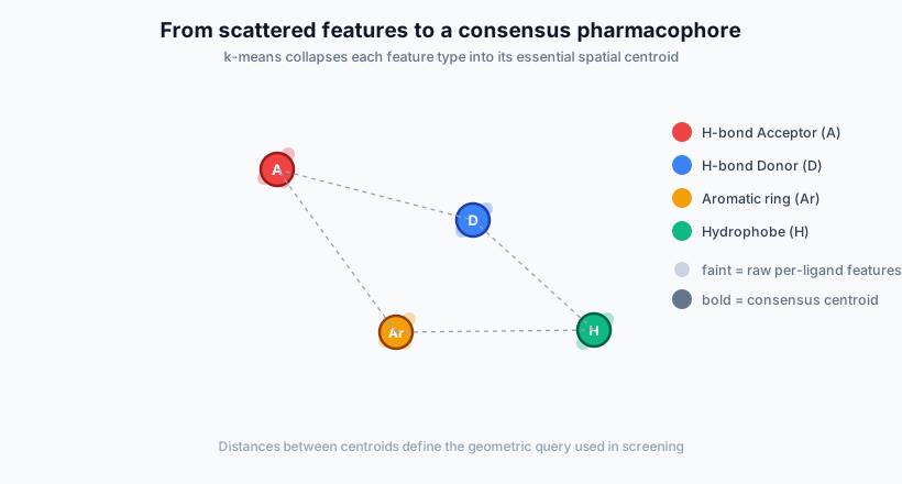
That cloud is the input. Group the points by family, donors with donors and acceptors with acceptors, and run k-means inside each family. The cluster count is
k = max(1, round(len(coords) / n_ligands)),
about one site per ligand. A centroid stays when members >= 0.5 * n_ligands.
import numpy as np
from collections import defaultdict
from sklearn.cluster import KMeans

# group every feature point by family
by_type = defaultdict(list)
for family, coord in all_features:
    by_type[family].append(coord)

n_ligands = len(target_cluster_ligands)
consensus = []

for family, coords in by_type.items():
    coords = np.array(coords)
    k = max(1, round(len(coords) / n_ligands))   # ~1 site per ligand
    km = KMeans(n_clusters=k, n_init="auto").fit(coords)

    for c in range(k):
        members = (km.labels_ == c).sum()
        # keep only features shared by the majority
        if members >= 0.5 * n_ligands:
            consensus.append((family, km.cluster_centers_[c]))

for family, center in consensus:
    print(f"{family:10s} at {np.round(center, 2)}")
The printout is a short list: family, then a center rounded to two decimals. Distances between those centers are the geometric query.
The payoff
The result is a 3D map of the features the overlaid ligands share, built from public structures and free libraries. Encode those features and the distances between them, then search ZINC, Enamine REAL, or an in-house collection for scaffolds that match the same pattern.
| Stage | Job | Tool |
|---|---|---|
| 1. Mine | Query and download QC-filtered structures | biotite + RCSB GraphQL |
| 2. Align | Parse and superpose pockets in 3D | MDAnalysis |
| 3. Cluster | Separate binding sites | scikit-learn (DBSCAN) |
| 4. Featurize | Fix bonds, extract features | RDKit (rdFMCS, FeatureFactory) |
| 5. Consensus | Distill the shared model | scikit-learn (k-means) |
Python and that stack are the whole chain. This note stops at the query.