Computational Strategies for Accelerating Drug Discovery: A Comprehensive Review
Abstract
Drug discovery is a complex and time-intensive process, often spanning over a decade and requiring substantial financial investments. Recent advances in cheminformatics and computational methods have revolutionized this field, enabling faster and more cost-effective approaches to identify and optimize drug candidates. This review highlights the role of cheminformatics in modern drug discovery, focusing on key methodologies such as quantitative structure-activity relationship (QSAR) modeling, molecular docking, and molecular dynamics simulations. We discuss the integration of artificial intelligence (AI) and machine learning (ML) algorithms for predictive modeling, virtual screening, and structure-based drug design, emphasizing their ability to handle large datasets and uncover hidden patterns. Key cheminformatics tools, including molecular fingerprints, pharmacophore modeling, and ligand-based screening, are explored for their application in lead optimization and target identification. The review also addresses the importance of chemical databases and molecular descriptors in enhancing predictive accuracy and outlines strategies for evaluating drug-likeness and ADMET profiles to improve candidate selection. Furthermore, we examine the role of molecular dynamics in capturing dynamic interactions and free-energy landscapes for ligand-protein complexes. Despite these advancements, challenges such as data standardization, model interpretability, and validation remain critical. By synthesizing recent developments and future directions, this review highlights the transformative potential of computational approaches in accelerating drug discovery while reducing costs and experimental failures.
Keywords: Cheminformatics, Drug Discovery, QSAR Modeling, Molecular Docking, Molecular Dynamics Simulations, Machine Learning, Artificial Intelligence, ADMET Prediction
Overview of the drug discovery process
The drug discovery process is a multifaceted journey that typically consists of several key stages. It often begins with a pre-discovery phase, where basic research is conducted to understand the mechanisms underlying diseases and identify potential targets, such as proteins [1]. Subsequently, the drug discovery stage involves the search for molecules, with a focus on small compounds that can modulate these targets. This process can involve the use of computer-aided drug design (CADD) approaches to identify and optimize potential drug candidates. CADD encompasses a range of theoretical and computational methods that are part of modern drug discovery, including structure-based drug design (SBDD) and ligand-based drug design (LBDD). These approaches employ mathematical tools and software packages to manipulate and quantify the properties of potential drug candidates, enabling the analysis of macromolecular structures and the prediction of their properties [2,3]. CADD has become an indispensable part of drug discovery, offering faster and more efficient drug design, a higher chance of success for improving drug efficacy, and a reduction in experimental costs [4]. The drug discovery process is a lengthy and rigorous endeavor, typically taking 10-15 years for a new drug to be approved. Throughout this process, various stages, such as target discovery, lead compound identification, and preclinical and clinical research, are undertaken to ensure the safety and effectiveness of potential drug candidates (Figure 1). The application of CADD in drug discovery has become increasingly important, offering valuable insights and guidance in the identification, optimization, and evaluation of potential drug candidates.
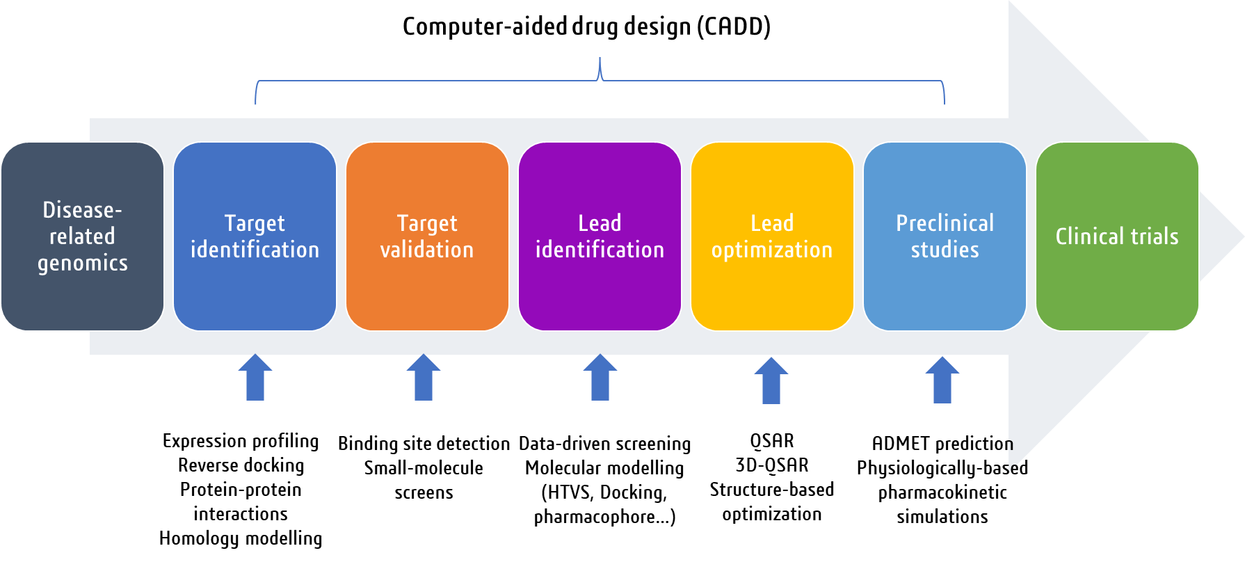
Figure 1. An overview of the main steps involved in the drug discovery process.
Cheminformatics in drug discovery
Cheminformatics emerged as an active field in the 1970s, initially in academia and later adopted by the pharmaceutical industry. The term was formally defined for drug discovery applications by F.K. Brown in 1998 [5]. It is an interdisciplinary field combining chemistry, computer science, and information science principles to solve chemical problems. Cheminformatics plays a pivotal role in drug discovery by aiding the design of compound libraries, chemical data storage, virtual screening, and quantitative structure-activity relationship (QSAR) modelling [6]. Data-driven drug discovery is an approach within cheminformatics that relies on analyzing large datasets to identify new therapeutic targets, optimize drug candidates, and improve drug discovery efficiency. It employs advanced computational techniques like ML and deep learning (DL) algorithms, and cheminformatics tools to process and extract insights from diverse data sources. This data-driven analysis aims to uncover intricate relationships between compound activity and chemical information, guiding and accelerating drug discovery efforts that would be challenging to achieve through traditional methods alone.
Quantitative structure-activity relationships
QSAR is the process by which a chemical structure is correlated with a well-determined effect, such as biological activity or pharmacokinetic property [7]. Thus, biological activity can be expressed quantitatively, such as the concentration of a substance required to achieve a certain biological response. Additionally, when physical and chemical properties or structures are expressed numerically, a mathematical relationship, or quantitative structure-activity relationship, can be proposed between them [7]. The mathematical expression obtained can then be used as a predictive means of the biological response for similar structures. QSAR models are constructed using ML algorithms, such as neural networks or decision trees (Figure 2). These algorithms are trained on known molecule data with measured biological activities, to predict the biological activity of new molecules [8]. QSAR models are often used in combination with other techniques, such as molecular modelling, to achieve better prediction accuracy. They can also be used to identify patterns in the data that can be used to understand the underlying mechanisms of biological activity. QSAR models are very useful for saving time and money by allowing for the prediction of biological activity of molecules before they are synthesized and tested in vitro or in vivo. However, they also have limitations and cannot always predict biological activity with high accuracy. Therefore, they should be used with caution and in combination with other techniques to achieve accurate results.
![Figure 2. Schematic representation of the QSAR modelling workflow [9].](/uploads/cdd-review/image2.png)
Figure 2. Schematic representation of the QSAR modelling workflow [9].
Chemical bioactivity databases
Chemical bioactivity databases such as ChEMBL, BindingDB, PubChem Bioassays, PDBbind, and BRENDA Enzyme Database play a crucial role in modern chemical biology research (Table 1). These databases contain curated data on experimental bioactive molecules including their chemical structures, bioactivity data (such as Ki, Kd, IC50, % of inhibition, and EC50), and interactions with macromolecules such as proteins and enzymes. These databases facilitate data-driven drug discovery approaches, such as applying ML methodologies to identify relationships in large datasets.
Table 1. List of popular open access chemical bioactivity databases used in drug discovery.
| Database | Advantages | Number of bioactivities | Website |
|---|---|---|---|
| ChEMBL | - Manually curated database of bioactive molecules ensuring high quality data - Comprehensive chemical and bioactivity data - Advanced filtering and analysis options |
>2.4 million compounds and >20 million activities | https://www.ebi.ac.uk/chembl/ |
| BindingDB | - Offers a public repository of experimental binding affinity data for protein-ligand interactions - Provides virtual screening tools to predict targets and identify potential drug candidates - Supports programmatic access and data downloads for integration into research workflows |
>1 million binding data points for >2,500 protein targets and ~500,000 small molecules | https://www.bindingdb.org/ |
| PubChem Bioassays | - Vast repository of chemical and biological data, including structures, bioactivities, and screening results - Search for molecules flexibly using names, SMILES codes, or chemical structures - Integrated analysis tools for exploring data patterns and relationships |
>1.5 million assay records, >115 million compounds and >290 million bioactivity data points | https://pubchem.ncbi.nlm.nih.gov/ |
| PDBbind | - Provides experimentally measured binding affinity data for protein-ligand complexes - Links energetic and structural information for detailed analysis of protein-ligand interactions - Requires free registration for full access to database, ensuring data security and access control |
Binding affinities for 23,496 biomolecular complexes in PDB, including protein-ligand (19,443), protein-protein (2,852), protein-nucleic acid (1,052), and nucleic acid-ligand complexes (149) | http://www.pdbbind.org.cn/ |
| BRENDA Enzyme Database | - Database focused on enzyme functions, providing comprehensive information on enzyme nomenclature, reactions, specificity, structure, and references - Offers data directly from primary literature, ensuring reliable and up-to-date information |
>330,000 enzyme synonyms, and >295,000 inhibitors, and >22,000 reactions | https://www.brenda-enzymes.org/ |
Molecular representations
The technological progress of the last century, marked by the computer revolution and the advent of high-throughput screening technologies in drug discovery, paved the way for computer analysis and visualization of bioactive molecules. To achieve this, it became necessary to represent molecules in a syntax that is readable by computers and understandable by scientists from various disciplines. Many chemical representations have been developed over the years, the number of which is due to the rapid development of computers and the complexity of producing a representation that encompasses all structural and chemical characteristics.
Graph representation
A molecular graph representation is a mapping of the atoms and bonds that make up a molecule into sets of nodes and edges. Typically, nodes are represented by circles or spheres, and edges by lines (Figure 3). In molecular graph representations, nodes are often represented using letters indicating the type of atom (like in the periodic table), or simply as the intersections of bonds (for carbon atoms) [10]. Formally, a molecular graph representation is a 2D object that can be used to represent 3D information (such as atomic coordinates, bond angles, and chirality). However, all spatial relationships between nodes must be encoded as node and/or edge attributes, as nodes in a graph (the mathematical object) do not formally have spatial positions, only pairwise relationships [11]. Both 2D and 3D representations of graphs can be easily visualized using various software programs, including UCSF Chimera, Avogadro, PyMOL, and VMD [12]
![Figure 3. Dopamine and its molecular graph: different node types according to atomic elements and different edge types depending on the chemical bond [13].](/uploads/cdd-review/image3.png)
Figure 3. Dopamine and its molecular graph: different node types according to atomic elements and different edge types depending on the chemical bond [13].
SMILES format
SMILES (Simplified Molecular Input Line Entry Specification) is a line notation language used to represent chemical structures as a string of ASCII characters (Figure 4). The language is designed to be simple, compact, and machine-readable, making it ideal for use in computer databases and for representing structures in computer programs [14]. SMILES can be used to store and analyze large amounts of molecular data, such as information about the structure of potential drug candidates. Additionally, SMILES can be used in conjunction with molecular modelling software to generate 2D and 3D representations of molecules, allowing researchers to perform molecular docking studies. These simulations can provide valuable information about the physical properties of potential drug candidates, such as their binding affinity, solubility, and stability [15].
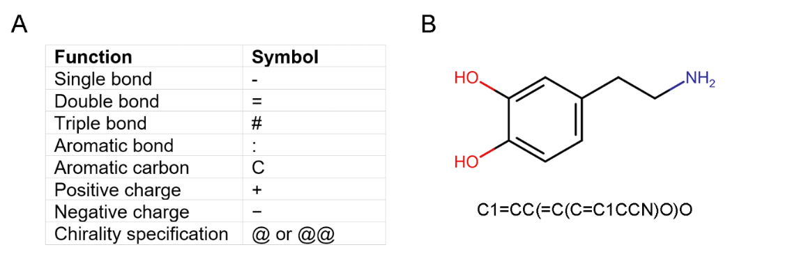
Figure 4. (A) Function and symbol of each ASCII character used in SMILES representation. (B) 2D chemical structure and SMILES representation of dopamine.
SMARTS format
SMARTS (SMILES arbitrary target specification) is a language used in cheminformatics to specify substructures in molecules. It is an extension of SMILES and allows for flexible and efficient substructure-search specifications in terms that are meaningful (Figure 5). SMARTS uses atomic and bond symbols to specify a graph, and the labels for the graph’s nodes and edges are used to say what type of atom each node represents and what type of bond each edge represents [16].
![Figure 5. SMARTS patterns and their visualization across three MACCS fingerprints using SMARTS PLUS [16].](/uploads/cdd-review/image5.png)
Figure 5. SMARTS patterns and their visualization across three MACCS fingerprints using SMARTS PLUS [16].
Connection tables
The MOL file format, created by MDL Information Systems, is part of the CT file family, also known as chemical table files (Figure 6). These files use connection tables to describe molecular structures, making them highly versatile and widely used for transferring chemical information. The MOL file format encapsulates the connection table and can be enclosed within a structure/data (SD) file, which includes not only structural information but also additional property data for multiple molecules. Other formats in the CT file family include the RXN file, which describes individual reactions, the RD file, which stores reactions or molecules along with their associated data, the RG file, designed for handling queries, and the XD file, an XML-based format for transferring structures or reactions with their metadata (Table 2) [17].
Table 2. Comparison between different connections tables formats.
| MOL format | MOL2 format | SDF format | RXN format |
|---|---|---|---|
| Can only store one molecule per file. Cannot store complex information. Need more storage space. Lack of explicit atom types. Lack of standardization. |
Store multiple records such as MOLECULE, ATOM, BOND, SUBSTRUCTURE, and SET. | Can store multiple chemical structures in one file. Can store other information (e.g. chemical properties). |
Used to store information on chemical reactions. |
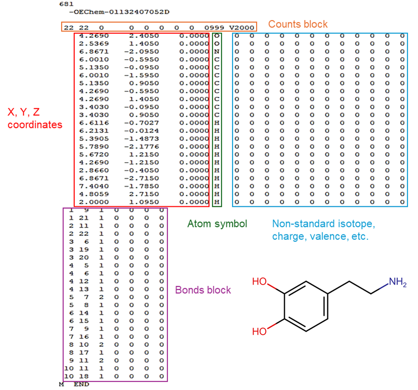
Figure 6. Representation of the connection tables for dopamine within an SDF file.
Molecular descriptors
A molecular descriptor in chemistry is a mathematical representation for characterizing a molecule that allows comparison of different molecules and searching for related molecules in a database [18]. These descriptors are classified into three categories: physicochemical, topological, or electronic, and are mostly characteristics of the 2D, or 3D structure of the molecule (Figure 7). The concept of “molecular descriptor” is closely related to the molecular structure and properties of an observable experimental molecule. The numerical values expressing the molecular descriptors can be obtained from the experimental physicochemical properties of the molecules or through theoretical mathematical formulas and computational algorithms [19].
![Figure 7. The different types of molecular descriptors [20].](/uploads/cdd-review/image7.png)
Figure 7. The different types of molecular descriptors [20].
Molecular fingerprints are descriptors specifically optimized for complex computational calculations, such as predictions of new properties using ML. These descriptors are encoded in 1D as bit vectors. The information represented by these bits can come from an initial 2D or 3D representation. In this work, we will focus on 2D molecular fingerprints, which are used to estimate the similarity between two molecules. These molecular fingerprints encode in each of their bits the presence or absence of certain substructures in the molecule. These fragments can be predefined or obtained from each molecule which is considered as a template. The Molecular ACCess System (MACCS) fingerprint is an example using predefined fragments. It consists of 166 substructures that can effectively distinguish between molecules [21]. The extended connectivity fingerprint (ECFP) is designed to capture the molecular features using a circle with an increasing diameter to obtain substructures representative of the molecule. The generation of an ECFP is illustrated in Figure 8. For example, the fingerprint has a length of 8 bits and the circles go up to a diameter of 4 atoms, taking the diameters of 0, 2 and 4 atoms. This diameter is commonly used for similarity search or molecule clustering. ML methods sometimes require higher diameters, up to 8 atoms. The length of the bit vector is usually much larger than the one used for the illustration, with a size of 1024 or 2048 bits [22].
![Figure 8. Generating an ECFP molecular fingerprint. The maximum allowed diameter is 4; successive circles have diameters of 0, 2 and 4. The presence of the obtained substructures is stored in a bit vector of length 8 [23].](/uploads/cdd-review/image8.jpeg)
Figure 8. Generating an ECFP molecular fingerprint. The maximum allowed diameter is 4; successive circles have diameters of 0, 2 and 4. The presence of the obtained substructures is stored in a bit vector of length 8 [23].
Artificial intelligence in drug discovery
Machine learning
ML models are increasingly being used to develop QSAR models, as they can handle large and complex datasets and can be used to identify patterns and relationships in the data that traditional statistical methods may not be able to detect (Figure 9). There are various ML models used in QSAR, such as Random Forest (RF), Support Vector Machine (SVM), k-Nearest Neighbors (KNN), and XGBoost (XGB) [24]. Among these, RF and SVM are considered the most widely used in drug discovery. RF is a type of ensemble learning method that combines multiple decision trees to improve the accuracy and stability of the model. It is particularly useful for handling high-dimensional and noisy data. SVM is a supervised learning algorithm that can be used for both classification and regression problems. It is particularly useful for handling small datasets with many features.
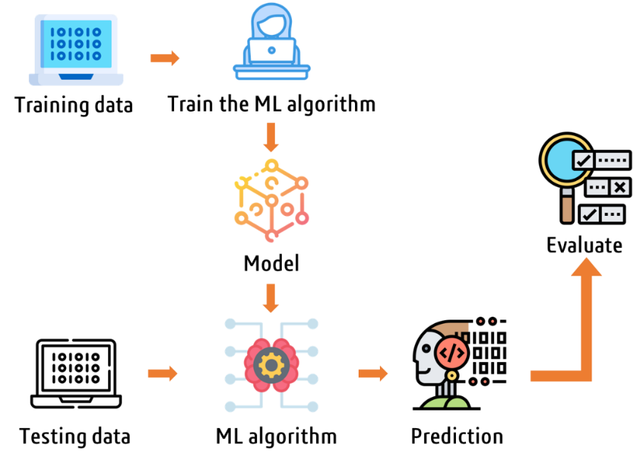
Figure 9. General workflow of a machine learning algorithm.
Random Forest
RF, developed by Leo Breiman in 2001, is an ensemble learning method used for classification, regression, and other tasks [25]. It operates by constructing multiple decision trees at training time, with each tree trained on a different subset of the data and using a random subset of features at each split [25]. The predictions of the individual trees are then combined to make the final prediction [26]. RF is known for its ability to handle overfitting by creating multiple trees, each trained slightly differently, which helps to reduce overfitting and improve the generalization performance of the model [27].
Support Vector Machine
SVM, firmly established by Vladimir Vapnik’s pioneering work and theoretical contributions, is a supervised learning algorithm specifically designed to identify a hyperplane that maximizes the margin between two distinct classes of data [28,29]. The margin is defined as the distance between the hyperplane and the nearest data points from each class [30]. These data points, which are near the hyperplane, are referred to as support vectors. Mathematically, the hyperplane is defined by the following equation (Eq. 1):
$$ w^{T} \times x + b = 0 \tag{1} $$Where $w$ is the normal vector to the hyperplane, $x$ is a data point, and $b$ is the bias term.
K-Nearest Neighbors
In 1919, Evelyn Fix proposed a nearest neighbor rule for estimating probability densities which was followed by progressive refinements culminating in its present-day prominence as a robust and versatile ML tool [31]. KNN algorithm is a non-parametric instance-based learning approach that classifies a new data point by examining the k nearest data points in the training set [32]. The label assigned to the new data point is determined by the most frequent class among its k nearest neighbors [33]. In most cases, the distance between two data points, $x$ and $y$, is computed using the Euclidean distance metric (Eq. 2):
$$ d(x, y) = \sqrt{\Sigma_{i}{(x_{i} - y_{i})}^{2}} \tag{2} $$Where $x_{i}$and $y_{i}$ are the $i$-th components of the data points x and y, respectively.
Gaussian Naïve Bayes
GNB is a classification technique used in ML based on a probabilistic approach and Gaussian distribution. It was developed by applying Bayes’ theorem with strong independence assumptions, making it an extension of the Naïve Bayes classifier [34]. GNB supports continuous-valued features and models each feature as conforming to a Gaussian distribution [35]. The mathematical representation of GNB is given by (Eq. 3):
$$ P(c|x) = \frac{(P(c) \times \prod P(xᵢ|c))}{P(x)} \tag{3} $$Where $P(c|x)$ is the probability of a data point ($x$) belonging to a specific class ($c$), given its features, $P(c)$ is the prior probability of class ($c$) being encountered, calculated from the overall frequency of class ($c$) in the dataset, $P(xᵢ|c)$ is the likelihood of observing a particular feature value ($xᵢ$) in data point ($x$) given that it belongs to class ($c$), and $P(x)$ is the overall probability of observing the data point ($x$), often calculated as a normalization factor to ensure probabilities sum to 1.
XGBoost
XGB, known as Extreme Gradient Boosting, represents a tree-based ensemble learning algorithm that operates within the framework of gradient boosting [36]. In 2014, Tianqi Chen’s vision set the spark for XGB, and thanks to Carlos Guestrin’s fine-tuning, it evolved into a powerhouse in the real world, boosting performance and pushing boundaries in the ML landscape [36]. This algorithm constructs a sequence of decision trees, with each subsequent tree trained to minimize the errors of its predecessors [36]. To mitigate overfitting, the trees undergo pruning. The predictions generated by an XGB model are the cumulative sum of the predictions made by all the trees within the ensemble (Eq. 4):
$$ ŷ = \Sigma_{t} \times f_{t}(x) \tag{4} $$Where $f_{t}\left( x \right)$is the prediction of the $t$*-*th tree for the data point $x$.
Deep learning
DL is a subset of ML that uses artificial neural networks with multiple layers to learn from large amounts of data and solve complex problems. It is based on the idea of representation learning and abstraction, where simple but non-linear modules transform the representation at one slightly more abstract level. DL models can create new features on their own and can be used to analyze various types of data, including images, voice, and text. DL has been increasingly applied to QSAR and quantitative structure-property relationship (QSPR) modelling, as it can handle complex data structures and interactions, and has shown promising results in predicting various properties of molecules [37].
Convolutional neural networks
A convolutional neural network (CNN) is a type of DL neural network that is designed to process data that has a grid-like topology, such as an image (Figure 10). CNNs are particularly useful for image recognition and classification tasks, as well as for natural language processing and speech recognition. In the context of drug discovery, CNNs can be used to develop QSAR/QSPR models. There are three main types of QSAR models that can be developed using CNNs: graph-based, image-based, and fingerprints-based models [38].
Graph-based QSAR models use the chemical structure of a compound represented as a graph, where atoms are nodes and chemical bonds are edges. CNNs can be used to learn the structural features of the compound from the graph representation [39].
For image-based QSAR models, CNNs can automatically extract relevant features and relationships from the molecular images. The convolutional layers enable the network to recognize spatial hierarchies of features, capturing important structural characteristics. This approach proves valuable in predicting the activity of compounds for drug discovery without the need for labor-intensive experiments.
In fingerprints-based QSAR models use the chemical structure of a compound represented as a binary fingerprint, where each bit corresponds to the presence or absence of a specific structural feature. CNNs can be used to learn the structural features of the compound from the fingerprint representation. Both types of models can be useful for drug discovery as they can predict the activity of compounds without the need for expensive and time-consuming experiments.
Several studies have explored the application of CNNs in QSAR modelling. For instance, a study published in the Journal of Cheminformatics introduced a molecular property prediction model based on the CNN framework, demonstrating the potential of deep learning in predicting molecular properties [40]. Additionally, a paper in the BMC Bioinformatics journal presented a learning-based method, CNN-DDI, for predicting drug-drug interactions using CNNs [41]. Furthermore, a study in Molecular Diversity journal discussed the potential of deep learning in improving QSAR models, highlighting the effectiveness of deep neural networks in learning directly from low-level encoded data without the need for computing molecular descriptors [42].
![Figure 10. The architecture of a convolutional neural network [43].](/uploads/cdd-review/image10.png)
Figure 10. The architecture of a convolutional neural network [43].
Artificial neural networks
Artificial neural networks (ANNs) are a type of ML algorithm that mimics the capacity of the human brain in terms of recognizing underlying relationships and patterns, mimicking the way the human brain processes information (Figure 11) [44]. ANNs can identify rules from samples and accurately describe the relationships between independent variables and dependent variables, and the training of ANNs resembles the process of approximating the formulas [45]. [46]. ANNs have been used in various drug discovery stages, including target identification, lead optimization, and toxicity prediction [46]. ANNs have also been used to develop QSAR models, which can predict the activity of compounds without the need for expensive and time-consuming experiments [46,47]. ANNs have been applied to drug discovery in various ways, such as predicting drug-related features, including bioactivities and drug-drug interactions, and accelerating the drug discovery process [38]. ANNs are crucial in medicinal chemistry for predicting and designing new molecules. They streamline drug discovery by enabling faster and more efficient drug design, increasing the likelihood of improving drug efficacy, and reducing experimental costs. [38,46,47].
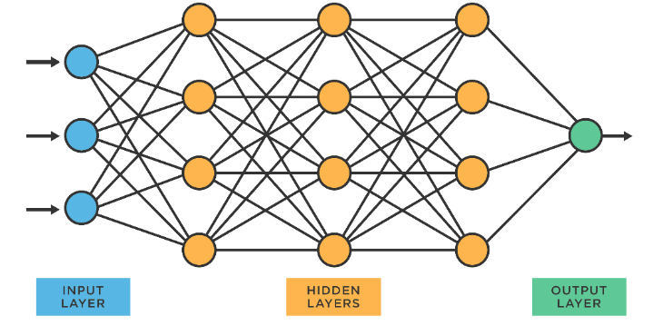
Figure 11. The architecture of an artificial neural network.
Recurrent neural networks
Recurrent neural networks (RNNs) have been successfully applied in drug discovery for de novo drug design, generating focused molecule libraries, and optimizing multiple traits collectively [48]. RNNs can learn the interrelationships between elements of the input over a protracted length of the input series, and they can capture sequential dependencies and generate new sequences based on learned patterns. According to recent research, Memory Augmented RNNs have been used for de novo drug design [49]. The study proposed three RNN-based architectures augmented with external memory for de-novo generation of small molecules. These architectures include a refactoring of a stack augmented RNN, adaptations of two recurrent neural network architectures, the Neural Turing Machine (NTM), and the Differentiable Neural Computer (DNC), with external memory to support random access, an advantage over the first-in-last-out access imposed by a stack and establishing their efficacy [49]. The study also compared the performance of these architectures with simpler recurrent neural networks (Long Short-Term Memory and Gated Recurrent Unit) without an external memory component to explore the impact of augmented memory in the task. The results showed that the proposed memory-augmented RNN architectures outperformed the baseline models in terms of the diversity and novelty of the generated molecules [49].
Performance evaluation
Regression metrics
In QSAR modelling, regression metrics are used to evaluate the performance of a regression model that predicts continuous numerical values, such as biological activity or property values, based on chemical features or descriptors of molecules.
Coefficient of determination.
The coefficient of determination (R2) is a measure of how well the regression model fits the data. It represents the proportion of the variance in the dependent variable that is predictable from the independent variable. The formula (Eq. 5) quantifies the proportion of the total variance in the dependent variable that is explained by the regression model. R2 values range from 0 to 1, where 1 indicates a perfect fit (the model explains all the variability), and values closer to 0 indicate poorer model fit.
$$ R² = 1 - (\frac{\text{SSres}}{\text{SStot}}) \tag{5} $$Where $\text{SSres}$ is the sum of squared residuals, also known as the residual sum of squares (RSS). It measures the total variance that is not explained by the regression model. $\text{SStot}$ is the total sum of squares, which represents the total variance in the dependent variable $\text{y }$around its mean.
Mean Squared Error.
The average squared difference between the predicted values and the actual values. It measures the overall prediction error of the model (Eq. 6).
$$ MSE = (\frac{1}{n}) \sum_{i = 1}^{n}{(y_{i} - ŷ_{i})}^{2} \tag{6} $$Where $n$ is the number of samples or observations. $y_{i}$represents the actual observed value for the 𝑖-th sample. $ŷ_{i}$ represents the predicted value for the 𝑖-th sample.
Mean Absolute Error.
The average absolute difference between the predicted values and the actual values (Eq. 7). It provides a more intuitive understanding of the prediction error than MSE.
$$ MAE = (\frac{1}{n}) \sum_{i = 1}^{n}{\left| y_{i} - ŷ_{i} \right| } \tag{7} $$Root Mean Squared Error.
The square root of the MSE. It has the same units as the dependent variable, making it easier to interpret than MSE (Eq. 8).
$$ RMSE = \sqrt{(\frac{1}{n}) \sum_{i = 1}^{n}{(y_{i} - ŷ_{i})}^{2}} \tag{8} $$Classification metrics
Classification metrics are used to evaluate the performance of models that predict categorical outcomes, such as the activity or toxicity of a molecule. These metrics assess how well the model predicts the class labels of the samples based on their chemical features or descriptors.
Sensitivity.
Sensitivity, also known as true positive rate or recall, measures the proportion of actual positive instances (true positives) that are correctly identified by the model as positive (Eq. 9). In other words, sensitivity quantifies the model’s ability to correctly detect or capture positive instances from the entire pool of positive instances in the dataset.
$$ SE = \frac{\text{TP}}{(TP + FN)} \tag{9} $$Where True Positives (TP) are the instances that are correctly classified as positive by the model. False Negatives (FN) are the instances that are actually positive but are incorrectly classified as negative by the model.
Specificity.
Specificity measures the proportion of true negative predictions (correctly predicted negatives) out of all actual negative instances in the dataset (Eq. 10).
$$ SP = \frac{\text{TN}}{(TN + FP)} \tag{10} $$Where True Negatives (TN) are the instances that are correctly classified as negative by the model. False Positives (FP) are the instances that are actually negative but are incorrectly classified as positive by the model.
Accuracy.
Accuracy measures the proportion of correctly classified instances out of the total number of instances (Eq. 11).
$$ ACC = \frac{(TP + TN)}{(TP + TN + FP + FN)} \tag{11} $$F1 Score.
The F1 score is the harmonic mean of precision and recall. It provides a single metric that balances both precision and recall (Eq. 12).
$$ F1 = \frac{2TP}{(2TP + FP + FN)} \tag{12} $$Matthews’ correlation coefficient.
Matthews’ correlation coefficient (MCC) is a metric commonly used to evaluate the performance of binary classification models, including those used in QSAR studies (Eq. 13). MCC considers true positives, true negatives, false positives, and false negatives, providing a balanced measure of classification performance, especially in imbalanced datasets.
$$ MCC = \frac{(TP \times TN - FP \times FN)}{\sqrt{((TP + FP) \times (TP + FN) \times (TN + FP) \times (TN + FN))}} \tag{13} $$Molecular modelling
Molecular modelling is a computational technique used to predict the properties and behavior of molecules. It encompasses various methods, theoretical and computational, that help researchers understand molecular systems and their processes [50]. The principles used in molecular modelling can be categorized into three main types: ab initio, empirical, and semi-empirical [51].
-
Ab initio methods: This approach is based on fundamental principles, which are derived from quantum mechanics. Ab initio MD is a type of ab initio molecular modelling that simulates the behavior of molecules in real time [52]. This method allows for the study of chemical processes in condensed phases with greater accuracy and fewer biases [52]. Density functional theory (DFT) is an example of ab initio calculations, instrumental in both de novo drug design and molecular geometry optimization [53]. In drug design, DFT aids in predicting stable structures, analyzing electronic properties, and assessing binding energies. For molecular geometry, DFT is used for optimization, transition state analysis, and vibrational studies, providing accurate insights into molecular behavior and interactions [54].
-
Empirical methods: This approach involves the use of force fields to describe the interactions between atoms in a molecule. The force fields are derived from experimental data, such as bond lengths, angles, and thermodynamic properties [55]. Empirical molecular modelling is often used in conjunction with MD simulations to study the conformational changes of proteins and the binding of ligands [55].
-
Semi-empirical methods: This approach combines the principles of quantum mechanics (QM) with experimental data to describe the electronic structure of molecules. Semi-empirical methods make approximations and use parameters fitted to experimental data, making them less computationally expensive than ab initio methods. While less fundamentally rigorous than ab initio, they can still provide reasonably accurate descriptions of molecular properties [51].
Molecular modelling techniques have been applied in various fields, including computational chemistry, drug design, computational biology, and materials science, to study molecular systems ranging from small chemical compounds to large biomolecules. These techniques have been instrumental in advancing our understanding of molecular processes and designing new molecules for therapeutic purposes [51].
Chemical libraries
Chemical libraries are collections of chemical compounds that are synthesized experimentally or isolated from natural sources such as plants, animals, and microorganisms. These compounds are often of interest for their potential medicinal properties, and many have been used for centuries in traditional medicine [56,57]. NP libraries can be created by isolating and purifying compounds from natural sources, or by synthesizing compounds that are structurally like those found in nature. These libraries can be used in a variety of applications, including drug discovery, material design, and chemical synthesis [58]. Chemical libraries are becoming increasingly important as a resource for drug discovery and development, as they can be used to screen large numbers of compounds for potential activity against specific targets. Table 3 presents a comprehensive compilation of publicly accessible libraries of NPs designed for virtual screening.
Table 3. Comprehensive list of natural product libraries suitable for high-throughput virtual screening studies.
| Database | Number of NPs | Description | Link |
|---|---|---|---|
| COCONUT | 406,747 | Contains curated, standardized data on natural product structures, bioactivities, origins, and references. | https://coconut.naturalproducts.net/ |
| LOTUS | 276,518 | Provides detailed information on NPs with known bioactivities and isolation information. | https://lotus.naturalproducts.net/ |
| ZINC20 | 80,617 | Includes both natural and synthetic compounds, ideal for virtual screening and cheminformatics research. | https://zinc20.docking.org/ |
| NPASS | 94,413 | Offers extensive data on natural product bioactivities, origins, and literature references. | https://bidd.group/NPASS/index.php |
| Cannabis Compound Database | 6,172 | Comprehensive resource for cannabinoids, terpenes, and other chemicals found in Cannabis sativa. | https://cannabisdatabase.ca/ |
| SuperNatural III | 449,058 | Features curated data on NPs with reported bioactivities and isolation details. | https://bioinf-applied.charite.de/supernatural_3/ |
| FooDB | 70,926 | Includes naturally occurring compounds found in food, particularly bioactive molecules. | https://foodb.ca/ |
| NANPDB | 4,928 | Focuses on NPs and traditional medicine knowledge from North African plants. | https://african-compounds.org/about/nanpdb/ |
| EANPDB | 1,871 | Focuses on NPs and traditional medicine knowledge from East African plants. | https://african-compounds.org/about/eanpdb/ |
| SANCDB | 1,017 | Focus on natural compounds isolated from the plant and marine life in and around South Africa | https://sancdb.rubi.ru.ac.za/ |
| CMNPD | 31,561 | Extensive resource for marine-derived NPs, including structures, bioactivities, and isolation sources. | https://www.cmnpd.org/ |
| SistematX | 8,593 | Provides data on plant secondary metabolites, including alkaloids, terpenoids, and phenolics. | https://sistematx.ufpb.br/ |
| Eximed | 5,096 | Features Natural-Product-Based Library with potential for drug development. | https://eximedlab.com/Screening-Compounds.html |
| CoumarinDB | 905 | Specialized database dedicated to coumarins, a class of NPs with diverse bioactivities. | https://yboulaamane.github.io/CoumarinDB/ |
| Ambinter | 11,648 | Comprehensive collection of NPs with structural and bioactivity information. | https://www.ambinter.com/ |
Ligand-based virtual screening
Ligand-based virtual screening is a method for predicting potential new active molecules based on the knowledge of at least one known active ligand. This approach relies on the principle that structurally similar molecules often exhibit similar bioactivity profiles. It proves particularly valuable in cases where the therapeutic target is unknown or lacks an experimentally resolved crystallographic structure. Furthermore, ligand-based virtual screening offers computational efficiency compared to structure-based approaches, enabling the screening of millions of compounds. The most employed methods include similarity search, pharmacophore modelling, and QSAR models. Additionally, 3D-QSAR, which incorporates knowledge of bioactive conformations for descriptor calculation, features techniques such as Comparative Molecular Field Analysis (CoMFA) and Comparative Molecular Similarity Indices Analysis (CoMSIA). These techniques aim to elucidate the spatial and steric requirements crucial for ligand-receptor interactions, optimizing molecular designs for enhanced bioactivity.
Similarity search
Similarity search is the method to use when very few ligands have been reported for the chosen biological target. A similarity search can be conducted as soon as an active ligand is known [59]. This method is based on the use of descriptors and similarity metrics to compare molecules to be screened against one or more reference ligands to predict their activity profile. Tanimoto similarity, also known as Tanimoto coefficient (Tc), is a similarity metric commonly used in cheminformatics to quantify the similarity between two molecular fingerprints. It is calculated as the ratio of the number of common bits (features) between two fingerprints to the total number of bits present in both fingerprints (Eq. 14). The Tanimoto index ranges from 0 (no common bits) to 1 (identical fingerprints). Several studies have shown that the Tanimoto index is a popular and effective choice for fingerprint-based similarity calculations [60].
$$ \text{Tc}_{(A,B)} = \frac{N(A \cap B)}{(N\left( A \right) + N\left( B \right) - N\left( A \cap B \right))} \tag{14} $$Where $N\left( A \right)$ is he number of bits set to 1 in molecule A’s fingerprint, $N\left( B \right)$ is the number of bits set to 1 in molecule B’s fingerprint, and $N\left( A \cap B \right)$ is the number of bits set to 1 in both molecule A and B’s fingerprints.
Pharmacophore modelling
The concept of pharmacophore was developed by Ehrlich in the late 19th century [61]. At that time, although the term pharmacophore was not used, Ehrlich developed the idea that certain chemical groups in a molecule are responsible for its biological or pharmacological action. The first modern definition of pharmacophore, using the term “abstract features” instead of “chemical groups”, dates to 1960 [62]. The first pharmacophore model identifying orders of magnitude of distance between the features constituting the pharmacophore (Figure 12a) was published in 1963 for muscarinic agents [63]. Kier also published the first pharmacophore model with precise distances measured between the different groups constituting the pharmacophore, referred to as the “proposed receptor pattern” (Figure 12b) [64].
![Figure 12. First published pharmacophores. Beckett’s model (a) from 1963 defines approximate distances between Zone 1 (anionic cavity), Zone 2 (positively charged), and Zone 3. Kier’s model (b) proposes calculated distances between three key atoms common to acetylcholine, muscarine, and muscarone [63,64].](/uploads/cdd-review/image12.jpeg)
Figure 12. First published pharmacophores. Beckett’s model (a) from 1963 defines approximate distances between Zone 1 (anionic cavity), Zone 2 (positively charged), and Zone 3. Kier’s model (b) proposes calculated distances between three key atoms common to acetylcholine, muscarine, and muscarone [63,64].
The official definition of International Union of Pure and Applied Chemistry (IUPAC) from 1998 states that a pharmacophore consists of the entire steric and electronic properties of a molecule that are necessary for optimal supramolecular interactions with a specific biological target, resulting in either generation or blocking of a biological response [65]. According to this definition, molecules sharing the same pharmacophore for a given target should bind to the receptor in an identical manner and exhibit similar activity profiles. The generated pharmacophore is then used to screen a chemical library for molecules that overlay with this pharmacophore. One of the major characteristics of this type of method is that a pharmacophore is defined by complementary pharmacophoric points, which are functional groups rather than groups of atoms. The different pharmacophoric points sought after include hydrogen bond donors and acceptors, positively charged groups that form electrostatic interactions with negatively charged groups and vice versa, and aromatic groups, considered separately from the larger class of hydrophobic groups from which they originate, and both are complementary to other hydrophobic groups [66].
Structure-based virtual screening
When the 3D structure of the biological target of interest is available, methods known as structure-based approaches can be used for virtual screening (Figure 13) [67]. These 3D structures can be obtained through two primary experimental methods:
-
X-ray crystallography: This technique involves crystallizing the protein and then bombarding it with X-rays to reveal its atomic structure.
-
Nuclear magnetic resonance (NMR): This method probes the protein’s structure in solution using magnetic fields and radio waves.
The resolution of a protein structure is a critical parameter in structural biology that describes the level of detail and precision with which the positions of atoms are determined.
A vast repository of experimentally determined 3D structures is freely accessible through the RCSB Protein Data Bank (PDB), a global resource housing over 200,000 structures to date [68]. Resolution is expressed in units of angstroms (Å) and is inversely related to the quality of the data. A lower resolution value indicates higher quality data, meaning that the crystallographers were able to obtain more detailed information about the atomic positions.
However, when experimental structures are unavailable, computational methods for structure prediction have become increasingly powerful:
-
Sequence homology modelling: This approach utilizes structural data from related proteins with known structures to construct a model of the target protein.
-
AlphaFold: This groundbreaking AI system, developed by DeepMind, has transformed structure prediction by achieving remarkable accuracy, often contrasting experimental methods [69]. AlphaFold (https://alphafold.ebi.ac.uk/) has generated over 200 million protein structures with high confidence, significantly expanding the structural coverage of the protein universe.
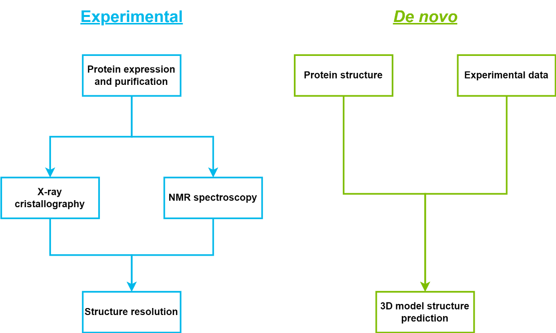
Figure 13. Methods to obtain the 3D structure of a biological target: experimental approaches (X-ray crystallography, NMR) and de novo methods (homology modelling, AlphaFold).
Concept of molecular docking
Over time, molecular docking has become an integral part of the drug discovery process. Since its initial development in the 1980s, advancements in computer hardware and the accessibility of small molecule and protein structures have contributed to the refinement of docking methods, resulting in its widespread adoption in both industrial and academic research [70]. The aim of molecular docking is to predict whether a molecule can bind to the active site of a protein based on the prediction of the conformation and orientation of the molecule during its binding to the receptor. To achieve this, docking methods combine the use of a search algorithm to generate putative binding modes or “poses” of the ligand in the receptor, and a scoring function used to rank the different poses according to a predicted affinity score. Docking methods aim to identify potential ligands of the protein target among all the molecules studied, and determine the correct poses or conformations adopted by the ligands during binding to the receptor.
Classification of molecular docking
For decades, the “lock-and-key” model dominated our understanding of ligand-receptor binding, leading to the development of rigid docking methods [71]. These early algorithms treated molecules as static entities, attempting to replicate the perfect key-hole fit [72]. In this approach, the ligand is positioned in the binding site through translation and rotation. For example, the software FRED enumerates all rotations and translations for a ligand inside the binding site as its first step[73]. Then, a negative image of the binding site is used to eliminate poses that are incompatible with the active site (due to clashes or distance). Finally, the selected poses are scored, and the best ones are optimized. However, this static view fails to capture the inherent dynamism of biomolecular interactions [73]. Figure 14 summarizes the differences between the three types of molecular docking.
Driven by the need for increased accuracy, semi-flexible docking emerged. This approach acknowledges the inherent conformational flexibility of both ligands and receptors, allowing limited conformational changes during the docking process [74]. Consequently, semi-flexible docking offers a more nuanced picture of binding by exploring a wider range of poses [75].. One common approach is to use a rotamer library to represent the possible conformations of the ligand [75]. The software then samples different combinations of rotamers and positions the ligand in the binding site. Another approach is to use a normal mode analysis to identify the most flexible regions of the ligand and the receptor [76]. The software then allows these regions to move during the docking simulation. However, for highly flexible systems, even semi-flexible approaches may fall short [77]. While computationally demanding, flexible docking provides unmatched accuracy, enabling the prediction of binding modes for complex and dynamic systems. One common approach is to use a protein structure prediction method to generate a library of receptor conformations [78]. The software then docks the ligand to each of these conformations and scores the resulting poses. Another approach is to use a MD simulation to simulate the binding process [79]. This allows the software to observe the ligand and receptor as they move and interact with each other.
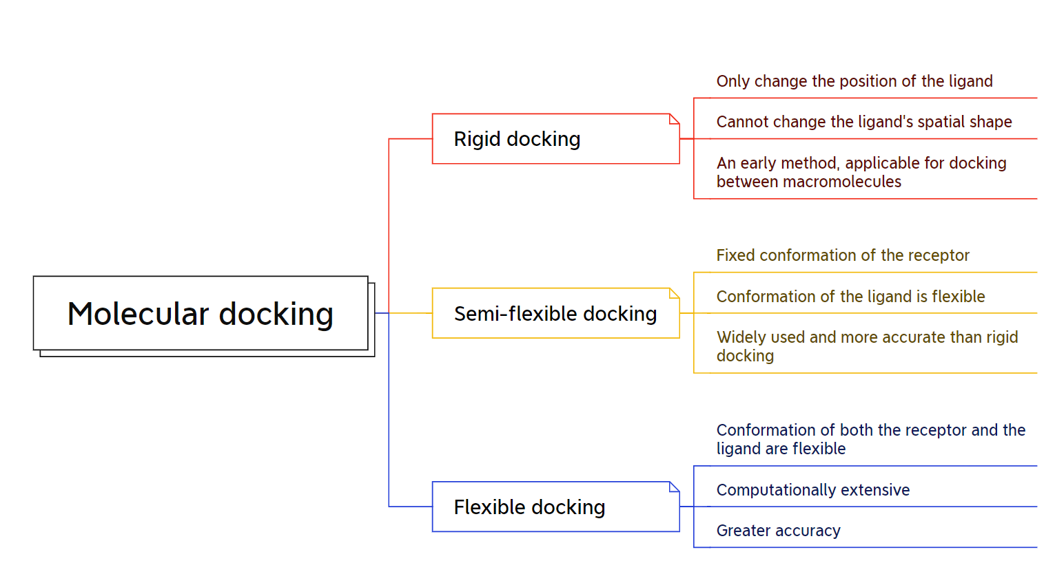
Figure 14. Molecular docking software classification.
Molecular docking programs
Molecular docking programs play a pivotal role in drug discovery, predicting the binding of small molecules to biomolecular targets. Through advanced algorithms, they simulate interactions and identify favorable binding modes, guiding the discovery of potent and selective drugs [80]. Virtual screening, enabled by molecular docking, efficiently prioritizes potential drug candidates from vast compound libraries, streamlining the drug discovery process. Continuous advancements, including refined force fields and flexibility considerations, further enhance docking programs, accelerating the path to new therapies. Table 4 provides information about different molecular docking programs, highlighting key aspects of each program.
Table 4. List of open-source and commercial molecular docking programs.
| Program | Licence | Docking Type | Scoring function | Reference |
|---|---|---|---|---|
| AutoDock Vina | Open-source | Flexible | Semi-empirical, force field-based, knowledge-based potentials | [81] |
| DOCK 4.0 | Open-source | Rigid, Semi-flexible | Empirical, force field-based scoring (grid-based) | [82] |
| GOLD | Commercial Academic | Flexible | Empirical (ChemScore, GoldScore, ChemPLP), knowledge-based function (ASP) |
[83] |
| Glide | Commercial | Flexible | Empirical (GlideScore, Ligand conformer (Emodel) | [84] |
| MOE | Commercial | Flexible | Empirical: London dG (fast and efficient, suitable for virtual screening), GBVI/WSA dG (more accurate, suitable for lead optimization) | [85] |
| AutoDock | Open-source | Flexible | Uses Lamarckian genetic algorithm. Semi-empirical, force field-based |
[86] |
| FlexX | Commercial | Flexible | Empirical | [87] |
| FRED | Academic | Rigid | Shape-based scoring, Chemgauss4 scoring | [88] |
| Surflex-Dock | Commercial | Flexible | Empirical scoring function | [89] |
| Molegro4 | Commercial | Flexible | Combines empirical, knowledge-based and force field scoring | [90] |
| Molegro5 | Open-source | Semi-flexible |
Docking screens protocol
High-throughput virtual screening (HTVS) is a computational technique that can rapidly sift through vast chemical libraries to identify a select number of molecules exhibiting desirable biological activity. HTVS enables the rapid evaluation of millions of compounds against target receptors. By assessing predicted binding affinities and modes, HTVS prioritizes candidate molecules with the highest potential for success, significantly narrowing the scope for subsequent wet-lab experimentation and optimizing resource allocation. This targeted approach not only enhances hit rates, but also mitigates the financial burden associated with late-stage clinical trial failures, which often stem from suboptimal lead compound selection.
The successful discovery of drugs heavily relies on the meticulous preparation of both the target protein and the candidate ligand for docking simulations (Figure 15). The protein structure undergoes necessary modifications including the addition of polar hydrogens and the removal of extraneous water molecules. Similarly, the ligand undergoes several preparations, including the addition of polar hydrogens, Gasteiger charge calculation, and the merging of non-polar atoms. Subsequently, the ligand is converted into a compatible format depending on the employed software. To define the search space for the binding site, a grid map is created. The docking run then evaluates various ligand poses within the binding site using a scoring function. The top-ranked candidates, typically within the top 10 %, are prioritized for further experimental validation and visualization with tools like Schrödinger’s PyMOL or UCSF Chimera.
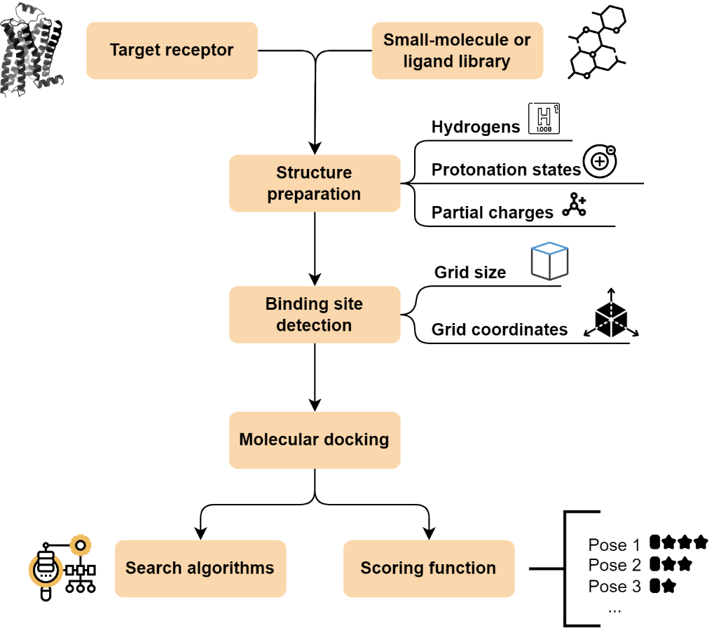
Figure 15. Flowchart of a molecular docking experiment.
Pharmacokinetics and toxicity filters
An estimated 40% of small-molecule drug candidates failing clinical trials in the 1990s suffered from poor bioavailability and pharmacokinetic properties, hindering their ability to reach target sites, and be effectively eliminated from the body (Figure 16) [91].
In the era of bioinformatics and cheminformatics, predictive tools have revolutionized drug discovery by allowing early prediction of drug-likeness and absorption, distribution, metabolism, elimination, and toxicity (ADMET) profiles of drug candidates. Despite the high costs associated with drug development, the pharmaceutical industry still faces a staggering 90% failure rate during the transition from preclinical to clinical trials [92,93].
![Figure 16. Evolution of the reasons for failure of drug candidates in clinical phases between 1991 and 2000 [94].](/uploads/cdd-review/image16.jpeg)
Figure 16. Evolution of the reasons for failure of drug candidates in clinical phases between 1991 and 2000 [94].
Physicochemical properties
Physicochemical properties are essential for understanding the probability of a drug candidate’s success and are used to filter compounds with unfavorable properties and poor development potential. Drug-likeness scores, which are based on physicochemical properties as shown in Figure 17, are used to assess a compound’s potential to succeed in clinical trials and are essential for economizing research costs. They are also a key element in raising the success of drug candidates during preclinical development. Physicochemical properties are related to interactions with different structural and physicochemical properties of drug candidates, and they are used to optimize drug-like properties of lead candidates. Certain physicochemical properties, such as molecular weight, are considered intrinsic properties of a molecule, meaning their values remain consistent regardless of the software used for their calculation. Other properties, however, are classified as predicted values and may exhibit slight variations between different software packages [95]. For example, Osiris Property Explorer and Marvin Suite water employ fragment-based methods to assign pre-calculated logS values to individual chemical fragments within the molecule and sum them up, accounting for bond adjustments and interactions. Other webservers like SwissADME use training datasets of known molecules and their logS values to statistically generate predictive QSPR models for calculating logS of new compounds.
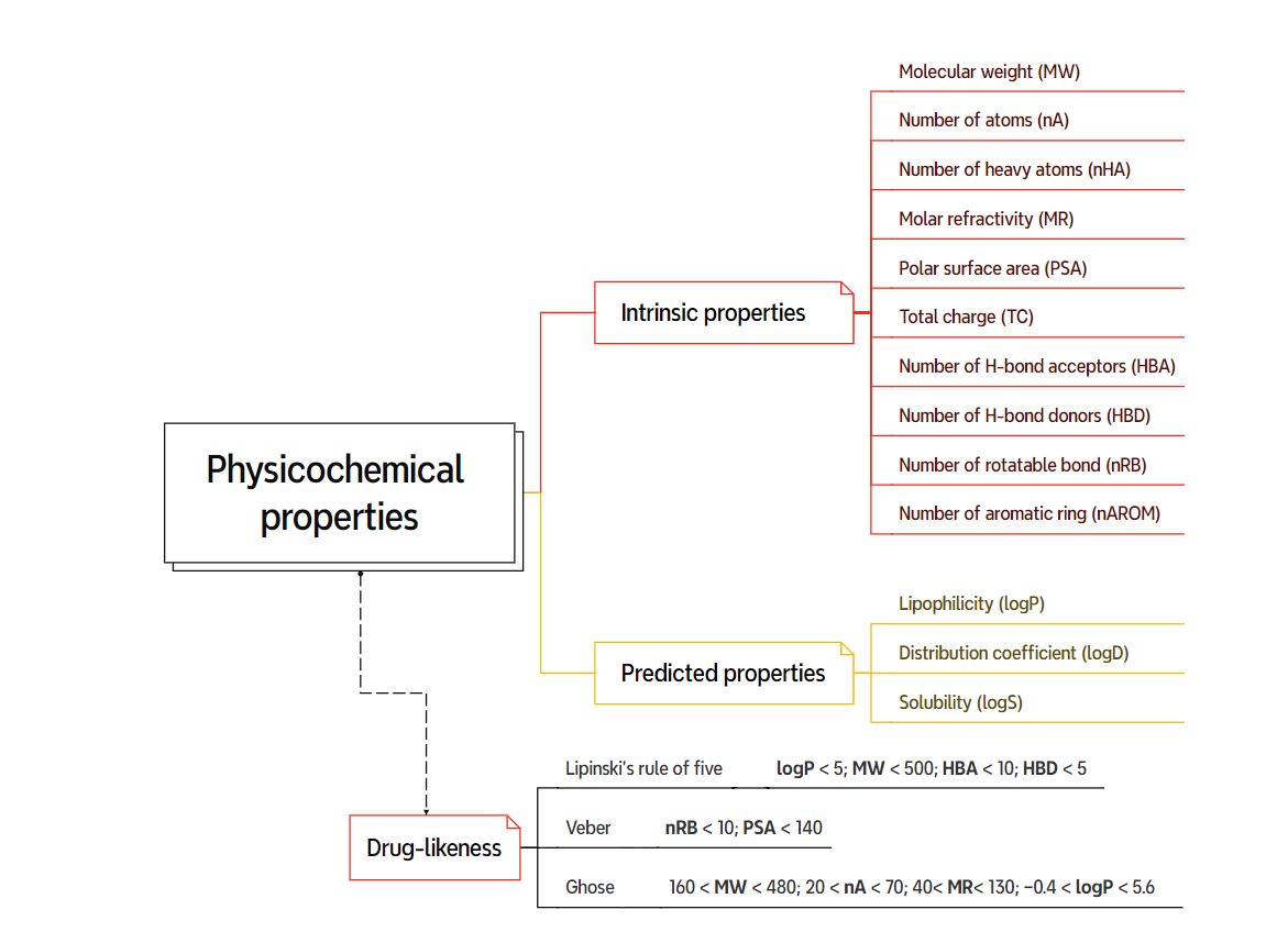
Figure 17. Commonly used physicochemical properties and their drug-likeness rules.
ADMET properties
The integration of ADMET profiling into early-stage drug synthesis represents a paradigm shift in the pharmaceutical landscape. Proactive optimization of these critical parameters has the potential to mitigate the risks and financial burdens associated with late-stage clinical trial failures, which often stem from suboptimal ADMET profiles. This shift is further empowered by the emergence of ML and AI-based QSPR models. These models, trained on extensive datasets of experimental ADMET data and molecular descriptors, enable the precise prediction of ADMET properties for novel drug candidates. This invaluable predictive power allows researchers to prioritize compounds with optimal absorption, distribution, metabolism, excretion, and toxicity profiles, streamlining the drug discovery process and boosting the success rate of promising therapeutics.
Furthermore, as detailed in Figure 18, specific physicochemical properties play a pivotal role in determining the in vivo fate and efficacy of drugs. Understanding these intricate relationships equips researchers with the knowledge to rationally design drug candidates with favourable ADMET characteristics, thereby accelerating the path towards safe and effective therapeutics for patients in need.
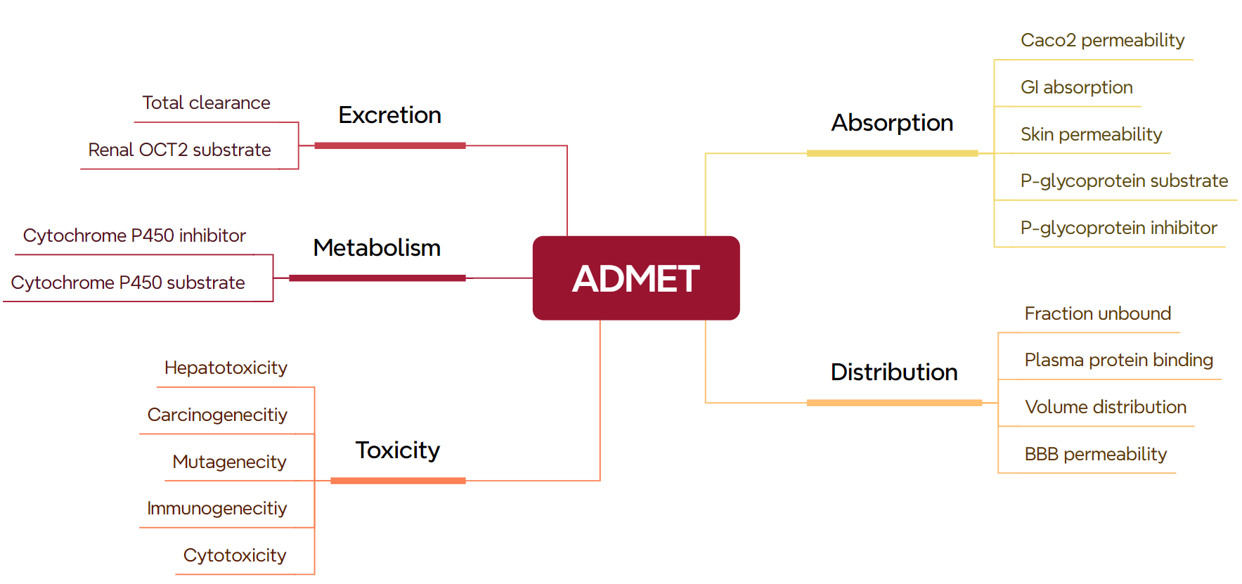
Figure 18. Visual diagram of key ADMET parameters for evaluating the safety of drug candidates during development.
In silico ADMET prediction tools
In silico ADMET tools are computational tools that can predict the ADMET properties of drug candidates using different mathematical models and algorithms, such as regression, classification, and neural networks [95]. In silico ADMET tools can predict various ADMET endpoints, such as Caco-2 permeability, BBB penetration, CYP450 interaction, and hepatotoxicity [96]. While in silico ADMET prediction tools have made significant progress, the accuracy and applicability of these tools depend on the quality and availability of experimental data, the validity and relevance of the models, and the user’s expertise and interpretation of the results. Some popular in silico ADMET tools include ADMETlab, SwissADME, and pkCSM, among others [97,98,99].
Molecular dynamics simulations
MD has emerged as an indispensable computational method, providing unprecedented insights into the dynamic behavior and intricate interactions of molecules. The field of structural biology has traditionally focused on capturing static snapshots of molecules, akin to frozen frames in a film. However, the essence of life lies in the dynamic interplay of atoms and molecules. MD serves as a bridge, simulating the time-dependent behavior of these microscopic entities and transforming static structures into dynamic systems.
Classical mechanics
Classical molecular mechanics (MM) forms the foundation of MD simulations, which are used to understand the motion and interactions of atoms and molecules. These simulations rely on the equations of classical mechanics, such as Newton’s laws of motion, to predict the positions and velocities of atoms at successive time steps. The basic principles of classical mechanics, like the conservation of energy and momentum, guide simulation dynamics. MD simulations are useful for studying large systems with a high number of particles, including protein-ligand complexes in drug discovery [100]. In comparison, Monte Carlo simulations provide an alternative approach. Unlike classical MD, Monte Carlo simulations use random sampling to explore the conformational space of molecules, focusing on thermodynamic ensembles and statistical probabilities [101]. This method is adept at studying systems with significant conformational changes, offering a statistical, thermodynamic perspective on the energetically favorable states of a system. Classical MD simulations have limitations stemming from the fact that they do not account for quantum effects and may not accurately represent the interactions between particles. Non-classical MD simulations, which uses forces obtained from electronic structure theory calculations (typically DFT) to evolve the system’s dynamics in time, can provide a more accurate representation of certain systems [102]. Despite these limitations, classical MD remains a valuable tool for investigating a wide range of biological and chemical phenomena, providing insights into the dynamic nature of molecular systems. Table 5 provides a comparative overview of Classical MD, ab initio simulations, and Monte Carlo simulations based on their underlying principles, representation of particles, time evolution approach, consideration of quantum effects, accuracy, typical applications, computational cost, and limitations.
Table 5. Comparison of Classical MD, ab initio simulations, and Monte Carlo simulations.
| Aspect | Classical MD | Ab Initio | Monte Carlo |
|---|---|---|---|
| Underlying Principles | Classical Mechanics | Quantum Mechanics | Statistical Mechanics |
| Particle Representation | Point masses for atoms and molecules | Explicit consideration of electron cloud | Statistical ensembles for molecular states |
| Time Evolution | Time-dependent trajectories of particles | Quantum mechanical evolution of wavefunctions | Statistical sampling of conformational space |
| Quantum Effects | Neglects quantum effects | Explicitly considers quantum effects | Does not consider quantum effects directly |
| Accuracy | Efficient for large systems, less accurate | High accuracy but computationally expensive | Statistical accuracy, less detailed trajectory |
| Applications | Macroscopic dynamics, large molecular systems | Small to medium-sized molecular systems | Wide range, especially for conformational studies |
| Computational Cost | Computationally efficient | Computationally expensive | Moderate computational cost |
| Typical Use Cases | Protein folding, ligand binding | Small molecules, electronic structure | Thermodynamics, conformational exploration |
| Limitations | Limited accuracy in capturing quantum effects | Computationally intensive for large systems | Limited in capturing detailed dynamic behavior |
Force fields
At the core of MD lies the concept of force fields, mathematical models that encapsulate the intricate web of interactions between atoms (Table 6). Force fields are vital in classical MD, defining a system’s potential energy surface and describing atomic and molecular interactions. These interactions include bonded terms (bond stretching, angle bending) and non-bonded terms (van der Waals forces, electrostatic interactions) [103,104]. Force field parameters are calibrated using experimental data and quantum calculations, influencing simulation outcomes [105]. Ongoing developments in force field refinement aim to address challenges like solvent effects and improve accuracy, enhancing the predictive capabilities of classical MD in capturing complex molecular system dynamics [106].
Table 6. Comparison of force fields in MD simulations.
| Force Field | Potential Energy Terms included | Description | Reference |
|---|---|---|---|
| AMBER | Bonded and non-bonded interactions | Biomolecules, proteins. Reproduces biomolecular structures well. Limited accuracy for some non-biological systems. | [107] |
| GAFF2 | Bonded and non-bonded interactions | Organic molecules, ligands. Improved accuracy for small organic molecules. May not be as accurate for large biomolecules and complex systems. | [108] |
| CHARMM36 | Bonded and non-bonded interactions | Biomolecules, lipids. Captures protein dynamics and lipid behavior. May require parameterization for non-standard molecules. | [109] |
| GROMOS | Bonded and non-bonded interactions | Biomolecules, small molecules. Efficient for small to medium-sized systems. Limited transferability to diverse molecular systems. | [110] |
| OPLS3e | Bonded and non-bonded interactions | Broad range of molecules. Balanced accuracy across various molecular types. Parameterization may be required for specific cases. | [111] |
| MARTINI | Coarse-grained representation | Lipids, polymers. Efficient for large-scale simulations, captures mesoscale behavior. Loss of atomic details, suitable for specific types of simulations. | [112] |
| AMOEBA | Many-body interactions, polarizability | Various molecular systems. Accurate representation of electrostatic and polar interactions. Computationally demanding, particularly for large systems. | [113] |
MD simulations workflow
Preparing and running MD simulation for a protein-ligand complex involves several key steps from system preparation to MD trajectory production.
System preparation
Each system is meticulously prepared to conform to the requirements of the selected force field. The nomenclature of atomic types and residue names is force field-specific, typically differing from that of the PDB. Notably, force fields exhibit distinctions in the protonation states of histidine, which are not explicitly captured in the PDB format. These states include charged state, neutral τ tautomer, anionic τ tautomer, and anionic π tautomer. Subsequently, any missing hydrogens are systematically added, and the hydrogen bonding network undergoes optimization. This optimization involves the rotation of the side chains of asparagine, glutamine, and histidine residues, or the adjustment of the protonation state in the case of histidines [114].
System solvation
Each protein-ligand complex is placed within a water box, which may take the form of a cubic, rectangular, triclinic, or orthorhombic shape. This configuration ensures a minimum water layer of at least 10 Å surrounds the complex. The choice of a water model, such as Single Point Charge (SPC) or Transferable Intermolecular Potential 3 Point (TIP3P), is crucial for accurately representing the behavior of water molecules in the simulation.
System neutralization
Additionally, the overall charge of the complex must be neutralized, this is achieved by adding Na+ and Cl− ions to the solvent. The electrostatic potential is computed at multiple points on a grid that spans the volume of the system, accounting for the positions of ions.
Energy minimization
The energy minimization step aims to optimize the molecular structure and reach a more stable starting configuration. It relieves steric clashes, corrects bond distortions, and allows the system to settle into a local energy minimum. During this step, an iterative optimization algorithm like steepest descent or conjugate gradient is used to adjust the atomic coordinates and minimize the potential energy of the system. Forces on atoms are calculated and positions are adjusted in each iteration until convergence criteria like an energy threshold or maximum iterations are met. The goal is to guide the system to a local minimum on the potential energy surface, where forces on each atom are near zero. After minimization, the stability and quality of the minimized structure are assessed by checking bond parameters, examining the overall structure, and ensuring no major clashes or unrealistic distortions remain. This step is crucial for obtaining a reasonable starting point for further calculations or simulations.
Equilibration
Following energy minimization, the equilibration step involves adjusting the system’s temperature and pressure, allowing solvent molecules to properly interact with the biomolecular components.
- NVT Equilibration (Constant Number of Particles, Volume, and Temperature): In the first equilibration phase, the system is allowed to evolve at a constant temperature (NVT ensemble). This involves applying a thermostat to control the temperature and adjusting atomic velocities accordingly. The duration of this phase allows the system to reach a thermal equilibrium, where the temperature fluctuations stabilize.
- NPT Equilibration (Constant Number of Particles, Pressure, and Temperature): Subsequently, the system undergoes equilibration at a constant temperature and pressure (NPT ensemble). This phase includes the application of a barostat to control pressure and may involve adjusting box dimensions to achieve the desired pressure. The system is allowed to equilibrate under these conditions, ensuring that both temperature and pressure fluctuations reach a stable state.
Production MD
Following NVT and NPT equilibration, the system transitions to the production MD run, where the dynamics of the protein-ligand complex are observed over an extended period. This phase is critical for obtaining meaningful data on the system’s behavior.
MD trajectory data analysis
In the analysis phase of the MD simulation, various techniques are employed to extract meaningful insights from the obtained trajectory data.
Root-Mean-Square Deviation
The Root-Mean-Square Deviation (RMSD) is a measure of the similarity between two structures. The RMSD between two structures $v$ and $w$ of $n$ atoms each (or $n$ points) is calculated with the following formula (Eq. 15):
$$ \text{RMSD}_{v,w} = \sqrt{\frac{1}{n}\sum_{i = 1}^{n}\left\| v_{i} - w_{i} \right\|^{2}} \tag{15} $$RMSD is used to compare protein structures. It is typically applied to the Cα atoms of the protein. In MD analysis, it is used to observe the deviation of the system from the initial structure. The system is equilibrated when the RMSD reaches a plateau. Other analyses are typically performed on the stabilized portion of the trajectory.
Root-Mean-Square Fluctuation
While RMSD is an average calculated over all atomic coordinates of the system at each step of the trajectory. The Root-Mean-Square Fluctuation (RMSF) corresponds to an average calculated over all steps of the trajectory for each atom (Eq. 16).
$$ \text{RMSF}_{i} = \sqrt{\frac{1}{T}\sum_{t = 0}^{t = T}\left( x_{i}^{t} - {x\bar{}}_{i} \right)^{2}} \tag{16} $$Here, $\text{RMSF}_{i}$represents the fluctuation of atom $i$ calculated over a trajectory of $T$ steps. It is determined by taking the square root of the average squared distance between the position of the atom at time t$(x_{i}^{t}$) and the average position of the atom (${x\bar{}}_{i}$). This analysis provides valuable insights into stable regions within protein structures.
Radius of gyration
The radius of gyration (Rg) is a measure of the compactness or spread of a molecular structure around its center of mass. Changes in Rag may indicate structural transitions, such as protein folding/unfolding or conformational changes induced by ligand binding or unbinding. Mathematically, the Rg can be expressed as (Eq. 17):
$$ Rg = \sqrt{\frac{1}{N}\sum_{i = 1}^{N}{m_{i}r_{i}^{2}}} \tag{17} $$Where $N$ is the total number of atoms, $m_{i}$is the mass of atom $i$, $r_{i}$ is the distance of atom $i$ from the centre of mass.
Solvent-accessible surface area
Solvent Accessible Surface Area (SASA) provides insights into the accessibility of a protein’s surface to its surrounding solvent environment. SASA quantifies the extent to which atoms on the protein surface are accessible to solvent molecules, influencing various biological processes, including ligand binding. Changes in SASA during protein-ligand interactions can indicate alterations in the protein’s conformation, accessibility of binding sites, and the potential impact on ligand binding affinity.
The Shrake-Rupley algorithm is widely employed for SASA calculations due to its computational efficiency. It involves rolling a probe sphere over the molecular surface and determining the solvent-accessible points, allowing for an estimation of the accessible surface area of the biomolecule.
Hydrogen bond analysis
Hydrogen bonds play a crucial role in maintaining the structure of proteins. The energy required to break a hydrogen bond ranges from 5 to 30 kJ/mol, making it stronger than van der Waals interactions but weaker than ionic or covalent bonds. Hydrogen bonds involve an electronegative atom such as oxygen, nitrogen, or fluorine, and a hydrogen atom covalently bonded to another electronegative atom.
The formation of a hydrogen bond depends on the relative position and the types of atoms in the donor (D) and acceptor (A). In MD simulations, observations on hydrogen bonds include the average number of bonds, which can be used to compare interactions between atom groups, and an analysis of occupancy or presence, providing information on stable regions within a molecule. Parameters such as the angle (θ) between the DH and DA vectors and the distance (d) between D and A are crucial, with θ being less than 40° and d less than 3.5 Å for effective hydrogen bonding as illustrated in Figure 19 [115].
![Figure 19. Geometric constraints of a hydrogen bond [115].](/uploads/cdd-review/image19.png)
Figure 19. Geometric constraints of a hydrogen bond [115].
Principal component analysis
Principal component analysis (PCA) is a powerful statistical method that aims to reduce the dimensionality of a dataset while retaining the essential features and variability present in the original data. In the context of MD simulations of biomolecular systems, PCA is particularly valuable for identifying dominant motions, describing structural variations, and uncovering the principal components governing the system’s dynamics.
-
Covariance Matrix: PCA begins by constructing the covariance matrix from the atomic positional fluctuations obtained during the MD simulation.
-
Eigen decomposition: The covariance matrix is then diagonalized, yielding eigenvectors and eigenvalues.
-
Principal Components: The eigenvectors represent the principal components, and the eigenvalues indicate the magnitude of the variance along each principal component.
Free energy calculations
Molecular mechanics/Generalized Born Surface Area
Molecular mechanics/Generalized Born Surface Area (MM/GBSA) is a computational approach used to estimate free energy changes in biomolecular systems, particularly for studying binding affinities of ligands to proteins [116]. The MM/GBSA method was developed by Peter Kollman and his group at the University of California, San Diego (UCSD) in the late 1990s [117]. It combines MM calculations, which describe the bonded and non-bonded interactions within the system, with a continuum solvation model based on the Generalized Born (GB) theory to account for solvent effects [118]. The binding free energy of a ligand to a protein receptor is calculated as the thermodynamic difference between the individual free energies of the free protein (P), the free ligand (L), and the formed complex (PL) in solvent (Eq. 18):
$$ \text{ΔG}_{\text{bind}} = G_{\text{PL}} - (G_{P} + G_{L}) \tag{18} $$The binding free energy can be decomposed into the vacuum potential energy, $\text{ΔE}_{\text{MM}}$, which includes the energy of both bonded as well as non-bonded interactions (Eq. 19), and it is calculated based on the MM force-field parameters [119,120].
$$ \text{ΔE}_{\text{MM}} = \text{ΔE}_{\text{bonded}} + \text{ΔE}_{\text{nonbonded}} = \text{ΔE}_{\text{bonded}} + ( \text{ΔE}_{\text{ele}} + \text{ΔE}_{\text{vdw}}) \tag{19} $$Where $\text{ΔE}_{\text{bonded}}$represents bonded interactions encompassing bond, angle, dihedral, and improper interactions. $\text{ΔE}_{\text{nonbonded}}$ represents nonbonded interactions comprising both electrostatic ($\text{ΔE}_{\text{ele}}$) and van der Waals ($\text{ΔE}_{\text{vdw}}$) interactions, modeled through Coulomb and Lennard-Jones potential functions, respectively. In the single trajectory approach, the conformation of the protein and ligand in both the bound and unbound forms is assumed to be identical. Consequently, $\text{ΔE}_{\text{bonded}}$is consistently considered as zero [121].
This binding free energy can be further described to account for the free energy of solvation (Eq. 20):
$$ \text{ΔG}_{\text{bind}} = \text{ΔE}_{\text{ele}} + \text{ΔE}_{\text{vdw}} + \text{ΔG}_{\text{GB}} + \text{ΔG}_{\text{SASA}} - T\Delta S \tag{20} $$The equation incorporates the solvation energy ($\text{ΔG}_{\text{GB}}$) accounting for polar solvation effects using an implicit solvation GB model, and the SASA solvation energy ($\text{ΔG}_{\text{SASA}}$) capturing nonpolar solvation effects based on the approximation of SASA [122]. The conformational entropy term ($- T\Delta S$) which is calculated by normal-mode analysis, is usually neglected due to the high computational cost and technical errors associated with its calculation [123].
Molecular mechanics/Poisson-Boltzmann Surface Area
Like MM/GBSA, Molecular mechanics/Poisson-Boltzmann Surface Area (MM/PBSA) is a computational method used for the estimation of free energy changes in biomolecular systems, especially for studying ligand binding to proteins. MM/PBSA combines MM calculations with a continuum solvation model as described in MM/GBSA (Eq. 21), but it uses the computationally time-consuming Poisson-Boltzmann (PB) equation to describe the electrostatic solvation effects ($\text{ΔG}_{\text{solv}})$ [124].
$$ \text{ΔG}_{\text{bind}} = \text{ΔE}_{\text{ele}} + \text{ΔE}_{\text{vdw}} + \text{ΔG}_{\text{solv}} + \text{ΔG}_{\text{SASA}} - T\Delta S \tag{21} $$MD simulations software
There are several software packages available for MD simulations. Some popular options include GROMACS, AMBER, Desmond, LAMMPS, and NAMD. These software packages are widely used for MD simulations and offer various features suitable for different research needs. GROMACS is a free and open-source software suite for high-performance MD and output analysis [125], while AMBER is a suite of programs for MD simulations of proteins and nucleic acids [126]. Desmond is a high-performance MD simulation software package developed at D. E. Shaw Research. It is designed to perform MD simulations of biological systems on conventional computer clusters and can also be used for absolute and relative free energy calculations, such as free energy perturbation [127]. LAMMPS is a classical MD code with a focus on materials modelling [128]. NAMD is a powerful, parallel MD simulation software package [129]. The choice of software depends on specific research requirements, user expertise, and the nature of the simulations to be performed. Table 7 details some of the commonly used MD simulation software packages.
Table 7. Description of commonly used software packages for MD simulations.
| Program | Licence | Description | Reference |
|---|---|---|---|
| GROMACS | Open-source (GPLv2) | A versatile package to perform MD, scalable and efficient in performing large-scale simulations | [125] |
| AMBER | Open-source (Artistic License 2.0) | A suite of biomolecular simulation programs that includes several force fields for the simulation of proteins, nucleic acids, and carbohydrates. | [126] |
| Desmond | Commercial and academic | Developed by Schrödinger, Desmond is a high-performance MD simulation program with a focus on drug discovery. | [127] |
| LAMMPS | Open-source (GPLv2) | A classical MD simulation code, designed to run efficiently on parallel computers. | [128] |
| NAMD | Open-source (NAMD License, like GPL) | A parallel MD code designed for high-performance simulation of large biomolecular systems. | [129] |
Conclusion
Cheminformatics and computational methods have become indispensable in modern drug discovery, significantly accelerating the identification and optimization of drug candidates while reducing costs and experimental failures. This review highlights the transformative impact of key methodologies such as QSAR modeling, molecular docking, molecular dynamics simulations, and ligand- and structure-based virtual screening. The integration of artificial intelligence and machine learning further enhances the predictive power and efficiency of these approaches, enabling the analysis of large datasets and uncovering complex structure-activity relationships.
Advancements in cheminformatics tools, molecular representations, and bioactivity databases have expanded the scope and depth of drug discovery pipelines. Moreover, the incorporation of ADMET profiling at early stages provides a more holistic evaluation of drug-likeness, optimizing the likelihood of clinical success. While these computational techniques offer immense potential, challenges such as data standardization, model validation, and limited interpretability of machine learning models persist.
Future efforts should focus on improving the integration of computational methods with experimental workflows, leveraging next-generation technologies like quantum computing and generative AI for de novo drug design. By addressing existing challenges and harnessing the synergy between computational and experimental approaches, researchers can continue to advance the development of safe, effective, and innovative therapeutics, ultimately transforming healthcare outcomes globally.
References
-
N. Singh, P. Vayer, S. Tanwar, J.-L. Poyet, K. Tsaioun, and B. O. Villoutreix, “Drug discovery and development: introduction to the general public and patient groups,” Frontiers in Drug Discovery, vol. 3, p. 1201419, May 2023, doi: 10.3389/FDDSV.2023.1201419.
-
W. Yu and A. D. Mackerell, “Computer-Aided Drug Design Methods,” Methods Mol Biol, vol. 1520, p. 85, 2017, doi: 10.1007/978-1-4939-6634-9_5.
-
J. P. Hughes, S. S. Rees, S. B. Kalindjian, and K. L. Philpott, “Principles of early drug discovery,” Br J Pharmacol, vol. 162, no. 6, p. 1239, Mar. 2011, doi: 10.1111/J.1476-5381.2010.01127.X.
-
P. Sharma, K. Sharma, and M. Nandave, “Computational approaches in drug discovery and design,” Computational Approaches in Drug Discovery, Development and Systems Pharmacology, pp. 53–93, Jan. 2023, doi: 10.1016/B978-0-323-99137-7.00009-5.
-
N. Brown, “Chemoinformatics—An Introduction for Computer Scientists,” ACM Comput Surv, vol. 41, no. 2, 2009, doi: 10.1145/1459352.1459353.
-
R. Guha and A. Bender, Computational Approaches in Cheminformatics and Bioinformatics. 2011. doi: 10.1002/9781118131411.
-
H. M. Patel et al., “Quantitative structure-activity relationship (QSAR) studies as strategic approach in drug discovery,” Medicinal Chemistry Research, vol. 23, no. 12, pp. 4991–5007, Jun. 2014, doi: 10.1007/S00044-014-1072-3/METRICS.
-
S. Kwon, H. Bae, J. Jo, and S. Yoon, “Comprehensive ensemble in QSAR prediction for drug discovery,” BMC Bioinformatics, vol. 20, no. 1, pp. 1–12, Oct. 2019, doi: 10.1186/S12859-019-3135-4/FIGURES/4.
-
C. Nantasenamat, “Best practices for constructing reproducible QSAR models,” Methods in Pharmacology and Toxicology, pp. 55–75, 2020, doi: 10.1007/978-1-0716-0150-1_3/COVER.
-
D. S. Wigh, J. M. Goodman, and A. A. Lapkin, “A review of molecular representation in the age of machine learning,” Wiley Interdiscip Rev Comput Mol Sci, vol. 12, no. 5, p. e1603, Sep. 2022, doi: 10.1002/WCMS.1603.
-
M. Yamada and M. Sugiyama, “Molecular Graph Generation by Decomposition and Reassembling,” ACS Omega, vol. 8, no. 22, pp. 19575–19586, Jun. 2023, doi: 10.1021/ACSOMEGA.3C01078/ASSET/IMAGES/LARGE/AO3C01078_0011.JPEG.
-
L. David, A. Thakkar, R. Mercado, and O. Engkvist, “Molecular representations in AI-driven drug discovery: a review and practical guide,” Journal of Cheminformatics 2020 12:1, vol. 12, no. 1, pp. 1–22, Sep. 2020, doi: 10.1186/S13321-020-00460-5.
-
S. N. Ilemo, D. Barth, O. David, F. Quessette, M. A. Weisser, and D. Watel, “Improving graphs of cycles approach to structural similarity of molecules,” PLoS One, vol. 14, no. 12, p. e0226680, Dec. 2019, doi: 10.1371/JOURNAL.PONE.0226680.
-
A. Veselinovic, J. Veselinovic, J. Zivkovic, and G. Nikolic, “Application of SMILES Notation Based Optimal Descriptors in Drug Discovery and Design,” Curr Top Med Chem, vol. 15, no. 18, pp. 1768–1779, Jun. 2015, doi: 10.2174/1568026615666150506151533.
-
M. Hirohara, Y. Saito, Y. Koda, K. Sato, and Y. Sakakibara, “Convolutional neural network based on SMILES representation of compounds for detecting chemical motif,” BMC Bioinformatics, vol. 19, no. 19, pp. 83–94, Dec. 2018, doi: 10.1186/S12859-018-2523-5/FIGURES/7.
-
C. Ehrt, B. Krause, R. Schmidt, E. S. R. Ehmki, and M. Rarey, “SMARTS.plus – A Toolbox for Chemical Pattern Design,” Mol Inform, vol. 39, no. 12, Dec. 2020, doi: 10.1002/MINF.202000216.
-
A. Dalby et al., “Description of several chemical structure file formats used by computer programs developed at Molecular Design Limited,” J Chem Inf Model, vol. 32, no. 3, p. 244, Feb. 1992, doi: 10.1021/ci00007a012.
-
S. Sahoo, C. Adhikari, M. Kuanar, and B. Mishra, “A Short Review of the Generation of Molecular Descriptors and Their Applications in Quantitative Structure Property/Activity Relationships,” Curr Comput Aided Drug Des, vol. 12, no. 3, pp. 181–205, May 2016, doi: 10.2174/1573409912666160525112114.
-
L. Xue and J. Bajorath, “Molecular Descriptors in Chemoinformatics, Computational Combinatorial Chemistry, and Virtual Screening,” Comb Chem High Throughput Screen, vol. 3, no. 5, pp. 363–372, Oct. 2012, doi: 10.2174/1386207003331454.
-
E. Bielska, X. Lucas, A. Czerwoniec, J. M. Kasprzak, K. H. Kaminska, and J. M. Bujnicki, “Virtual screening strategies in drug design–methods and applications,” journals.pan.pl, vol. 92, pp. 249–264, 2011, Accessed: Feb. 09, 2023.
\[Online\]. Available: https://journals.pan.pl/Content/82320/mainfile.pdf
-
J. L. Durant, B. A. Leland, D. R. Henry, and J. G. Nourse, “Reoptimization of MDL Keys for Use in Drug Discovery,” J Chem Inf Comput Sci, vol. 42, no. 6, pp. 1273–1280, Nov. 2002, doi: 10.1021/CI010132R.
-
D. Rogers and M. Hahn, “Extended-connectivity fingerprints,” J Chem Inf Model, vol. 50, no. 5, pp. 742–754, May 2010, doi: 10.1021/CI100050T/ASSET/IMAGES/MEDIUM/CI-2010-00050T_0018.GIF.
-
G. Peyrat, “Conception d’inhibiteurs de protéines kinases à partir de méthodes in silico basées sur les fragments,” 2021. Accessed: Feb. 11, 2023.
\[Online\]. Available: https://theses.hal.science/tel-03921639/
-
Z. Wu et al., “Do we need different machine learning algorithms for QSAR modeling? A comprehensive assessment of 16 machine learning algorithms on 14 QSAR data sets,” Brief Bioinform, vol. 22, no. 4, Jul. 2021, doi: 10.1093/BIB/BBAA321.
-
L. Breiman, “Random forests,” Mach Learn, vol. 45, no. 1, pp. 5–32, Oct. 2001, doi: 10.1023/A:1010933404324/METRICS.
-
J. Ali, R. Khan, N. Ahmad, and I. Maqsood, “Random Forests and Decision Trees,” 2012, Accessed: Dec. 28, 2023.
\[Online\]. Available: www.IJCSI.org
-
T. K. Ho, “The random subspace method for constructing decision forests,” IEEE Trans Pattern Anal Mach Intell, vol. 20, no. 8, pp. 832–844, 1998, doi: 10.1109/34.709601.
-
W. S. Noble, “What is a support vector machine?,” Nature Biotechnology 2006 24:12, vol. 24, no. 12, pp. 1565–1567, Dec. 2006, doi: 10.1038/nbt1206-1565.
-
V. Vapnik and R. Izmailov, “Reinforced SVM method and memorization mechanisms,” Pattern Recognit, vol. 119, p. 108018, Nov. 2021, doi: 10.1016/J.PATCOG.2021.108018.
-
K. Q. Weinberger, J. Blitzer, and L. K. Saul, “Distance Metric Learning for Large Margin Nearest Neighbor Classification,” Adv Neural Inf Process Syst, vol. 18, 2005.
-
X. Hu, J. Wang, L. Wang, and K. Yu, “K-Nearest Neighbor Estimation of Functional Nonparametric Regression Model under NA Samples,” Axioms 2022, Vol. 11, Page 102, vol. 11, no. 3, p. 102, Feb. 2022, doi: 10.3390/AXIOMS11030102.
-
G. Guo, H. Wang, D. Bell, Y. Bi, and K. Greer, “KNN model-based approach in classification,” Lecture Notes in Computer Science (including subseries Lecture Notes in Artificial Intelligence and Lecture Notes in Bioinformatics), vol. 2888, pp. 986–996, 2003, doi: 10.1007/978-3-540-39964-3_62/COVER.
-
S. Zhang, X. Li, M. Zong, X. Zhu, and D. Cheng, “Learning k for kNN Classification,” ACM Transactions on Intelligent Systems and Technology (TIST), vol. 8, no. 3, Jan. 2017, doi: 10.1145/2990508.
-
H. Kamel, D. Abdulah, and J. M. Al-Tuwaijari, “Cancer Classification Using Gaussian Naive Bayes Algorithm,” Proceedings of the 5th International Engineering Conference, IEC 2019, pp. 165–170, Jun. 2019, doi: 10.1109/IEC47844.2019.8950650.
-
S. Alkhushayni, D. Al-Zaleq, L. Andradi, and P. Flynn, “The Application of Differing Machine Learning Algorithms and Their Related Performance in Detecting Skin Cancers and Melanomas,” J Skin Cancer, vol. 2022, 2022, doi: 10.1155/2022/2839162.
-
T. Chen and C. Guestrin, “XGBoost: A scalable tree boosting system,” Proceedings of the ACM SIGKDD International Conference on Knowledge Discovery and Data Mining, vol. 13-17-August-2016, pp. 785–794, Aug. 2016, doi: 10.1145/2939672.2939785.
-
V. Kotu and B. Deshpande, “Deep Learning,” Data Science, pp. 307–342, 2019, doi: 10.1016/B978-0-12-814761-0.00010-1.
-
H. Askr, E. Elgeldawi, H. Aboul Ella, Y. A. M. M. Elshaier, M. M. Gomaa, and A. E. Hassanien, “Deep learning in drug discovery: an integrative review and future challenges,” Artif Intell Rev, vol. 56, no. 7, pp. 5975–6037, Jul. 2023, doi: 10.1007/S10462-022-10306-1/FIGURES/3.
-
D. Jiang et al., “Could graph neural networks learn better molecular representation for drug discovery? A comparison study of descriptor-based and graph-based models,” J Cheminform, vol. 13, no. 1, pp. 1–23, Dec. 2021, doi: 10.1186/S13321-020-00479-8/FIGURES/6.
-
P. Karpov, G. Godin, and I. V. Tetko, “Transformer-CNN: Swiss knife for QSAR modeling and interpretation,” J Cheminform, vol. 12, no. 1, pp. 1–12, Mar. 2020, doi: 10.1186/S13321-020-00423-W/FIGURES/9.
-
C. Zhang, Y. Lu, and T. Zang, “CNN-DDI: a learning-based method for predicting drug–drug interactions using convolution neural networks,” BMC Bioinformatics, vol. 23, no. 1, pp. 1–11, Jan. 2022, doi: 10.1186/S12859-022-04612-2/FIGURES/3.
-
C. Hung and G. Gini, “QSAR modeling without descriptors using graph convolutional neural networks: the case of mutagenicity prediction,” Mol Divers, vol. 25, no. 3, pp. 1283–1299, Aug. 2021, doi: 10.1007/S11030-021-10250-2/METRICS.
-
Y. Boulaamane et al., “Exploring natural products as multi-target-directed drugs for Parkinson’s disease: an in-silico approach integrating QSAR, pharmacophore modeling, and molecular dynamics simulations,” J Biomol Struct Dyn, 2023, doi: 10.1080/07391102.2023.2260879.
-
J. Jiménez-Luna, F. Grisoni, and G. Schneider, “Drug discovery with explainable artificial intelligence,” Nature Machine Intelligence 2020 2:10, vol. 2, no. 10, pp. 573–584, Oct. 2020, doi: 10.1038/s42256-020-00236-4.
-
Y. Xu, X. Li, H. Yao, and K. Lin, “Neural networks in drug discovery: current insights from medicinal chemists,” https://doi.org/10.4155/fmc-2019-0118, vol. 11, no. 14, pp. 1669–1672, Jul. 2019, doi: 10.4155/FMC-2019-0118.
-
V. Mandlik, P. R. Bejugam, and S. Singh, “Application of Artificial Neural Networks in Modern Drug Discovery,” Artificial Neural Network for Drug Design, Delivery and Disposition, pp. 123–139, Jan. 2016, doi: 10.1016/B978-0-12-801559-9.00006-5.
-
D. Paul, G. Sanap, S. Shenoy, D. Kalyane, K. Kalia, and R. K. Tekade, “Artificial intelligence in drug discovery and development,” Drug Discov Today, vol. 26, no. 1, p. 80, Jan. 2021, doi: 10.1016/J.DRUDIS.2020.10.010.
-
M. H. S. Segler, T. Kogej, C. Tyrchan, and M. P. Waller, “Generating focused molecule libraries for drug discovery with recurrent neural networks,” ACS Cent Sci, vol. 4, no. 1, pp. 120–131, Jan. 2018, doi: 10.1021/ACSCENTSCI.7B00512/SUPPL_FILE/OC7B00512_SI_002.ZIP.
-
N. Suresh, N. C. A. Kumar, S. Subramanian, and G. Srinivasa, “Memory augmented recurrent neural networks for de-novo drug design,” PLoS One, vol. 17, no. 6, Jun. 2022, doi: 10.1371/JOURNAL.PONE.0269461.
-
O. Silakari and P. K. Singh, “Fundamentals of molecular modeling,” Concepts and Experimental Protocols of Modelling and Informatics in Drug Design, pp. 1–27, 2021, doi: 10.1016/B978-0-12-820546-4.00001-5.
-
J.-L. Rivail, “Molecular Modelling. Semi-Empirical and Empirical Methods of Theoretical Chemistry,” Computational Advances in Organic Chemistry: Molecular Structure and Reactivity, pp. 229–259, 1991, doi: 10.1007/978-94-011-3262-6_4.
-
R. Iftimie, P. Minary, and M. E. Tuckerman, “Ab initio molecular dynamics: Concepts, recent developments, and future trends,” Proc Natl Acad Sci U S A, vol. 102, no. 19, pp. 6654–6659, May 2005, doi: 10.1073/PNAS.0500193102/SUPPL_FILE/00193FIG5.JPG.
-
R. J. Bartlett, V. F. Lotrich, and I. V. Schweigert, “Ab initio density functional theory: the best of both worlds?,” J Chem Phys, vol. 123, no. 6, Aug. 2005, doi: 10.1063/1.1904585.
-
M. Hoffmann and J. Rychlewski, “Density Functional Theory (DFT) and Drug Design,” Reviews of Modern Quantum Chemistry, pp. 1767–1803, Dec. 2002, doi: 10.1142/9789812775702_0058.
-
“Fundamental Principles of Molecular Modeling,” Fundamental Principles of Molecular Modeling, 1996, doi: 10.1007/978-1-4899-0212-2.
-
M. Sorokina, P. Merseburger, K. Rajan, M. A. Yirik, and C. Steinbeck, “COCONUT online: Collection of Open Natural Products database,” J Cheminform, vol. 13, no. 1, pp. 1–13, Dec. 2021, doi: 10.1186/S13321-020-00478-9/FIGURES/4.
-
Y. Boulaamane, P. Kandpal, A. Chandra, M. R. Britel, and A. Maurady, “Chemical library design, QSAR modeling and molecular dynamics simulations of naturally occurring coumarins as dual inhibitors of MAO-B and AChE,” J Biomol Struct Dyn, 2023, doi: 10.1080/07391102.2023.2209650.
-
B. A. P. Wilson, C. C. Thornburg, C. J. Henrich, T. Grkovic, and B. R. O’Keefe, “Creating and screening natural product libraries,” Nat Prod Rep, vol. 37, no. 7, pp. 893–918, Jul. 2020, doi: 10.1039/C9NP00068B.
-
H. Koeppen, J. Kriegl, U. Lessel, C. S. Tautermann, and B. Wellenzohn, “Ligand-Based Virtual Screening,” pp. 61–85, May 2011, doi: 10.1002/9783527633326.CH3.
-
D. Bajusz, A. Rácz, and K. Héberger, “Why is Tanimoto index an appropriate choice for fingerprint-based similarity calculations?,” J Cheminform, vol. 7, no. 1, pp. 1–13, Dec. 2015, doi: 10.1186/S13321-015-0069-3/FIGURES/7.
-
O. F. Güner and J. P. Bowen, “Setting the record straight: The origin of the pharmacophore concept,” J Chem Inf Model, vol. 54, no. 5, pp. 1269–1283, Apr. 2014, doi: 10.1021/CI5000533/ASSET/IMAGES/MEDIUM/CI-2014-000533_0002.GIF.
-
X. Qing et al., “Pharmacophore modeling: advances, limitations, and current utility in drug discovery,” Journal of Receptor, Ligand and Channel Research , vol. 7, pp. 81–92, Jan. 2014, doi: 10.2147/JRLCR.S46843.
-
A. H. Beckett, N. J. Harper, and J. W. Clitherow, “The Importance of Stereoisomerism in Muscarinic Activity,” Journal of Pharmacy and Pharmacology, vol. 15, no. 1, pp. 362–371, Apr. 2011, doi: 10.1111/J.2042-7158.1963.TB12799.X.
-
L. B. Kier, “Molecular Orbital Calculation of Preferred Conformations of Acetylcholine, Muscarine, and Muscarone,” Mol Pharmacol, vol. 3, no. 5, 1967.
-
D. R. Buckle et al., “Glossary of terms used in medicinal chemistry. Part II (IUPAC recommendations 2013),” Pure and Applied Chemistry, vol. 85, no. 8, pp. 1725–1758, Jul. 2013, doi: 10.1351/PAC-REC-12-11-23/MACHINEREADABLECITATION/RIS.
-
F. R. Makhouri and J. B. Ghasemi, “Combating Diseases with Computational Strategies Used for Drug Design and Discovery,” Curr Top Med Chem, vol. 18, no. 32, pp. 2743–2773, Mar. 2019, doi: 10.2174/1568026619666190121125106.
-
L. Maveyraud and L. Mourey, “Protein X-ray Crystallography and Drug Discovery,” Molecules, vol. 25, no. 5, Feb. 2020, doi: 10.3390/MOLECULES25051030.
-
A. Kouranov et al., “The RCSB PDB information portal for structural genomics,” Nucleic Acids Res, vol. 34, no. suppl_1, pp. D302–D305, Jan. 2006, doi: 10.1093/NAR/GKJ120.
-
J. Jumper et al., “Highly accurate protein structure prediction with AlphaFold,” Nature 2021 596:7873, vol. 596, no. 7873, pp. 583–589, Jul. 2021, doi: 10.1038/s41586-021-03819-2.
-
F. Stanzione, I. Giangreco, and J. C. Cole, “Use of molecular docking computational tools in drug discovery,” Prog Med Chem, vol. 60, pp. 273–343, Jan. 2021, doi: 10.1016/BS.PMCH.2021.01.004.
-
“Molecular docking towards drug discovery - Gschwend - 1996 - Journal of Molecular Recognition - Wiley Online Library.” Accessed: Dec. 11, 2023.
\[Online\]. Available: https://onlinelibrary.wiley.com/doi/10.1002/(SICI)1099-1352(199603)9:2%3C175::AID-JMR260%3E3.0.CO;2-D
-
N. Sauton, D. Lagorce, B. O. Villoutreix, and M. A. Miteva, “MS-DOCK: Accurate multiple conformation generator and rigid docking protocol for multi-step virtual ligand screening,” BMC Bioinformatics, vol. 9, no. 1, pp. 1–12, Apr. 2008, doi: 10.1186/1471-2105-9-184/FIGURES/3.
-
M. McGann, “FRED pose prediction and virtual screening accuracy,” J Chem Inf Model, vol. 51, no. 3, pp. 578–596, Mar. 2011, doi: 10.1021/CI100436P/SUPPL_FILE/CI100436P_SI_001.PDF.
-
J. Fan, A. Fu, and L. Zhang, “Progress in molecular docking,” Quantitative Biology, vol. 7, no. 2, pp. 83–89, Jun. 2019, doi: 10.1007/S40484-019-0172-Y/METRICS.
-
F. Ding, S. Yin, and N. V. Dokholyan, “Rapid flexible docking using a stochastic rotamer library of ligands,” J Chem Inf Model, vol. 50, no. 9, pp. 1623–1632, Sep. 2010, doi: 10.1021/CI100218T/ASSET/IMAGES/MEDIUM/CI-2010-00218T_0010.GIF.
-
C. N. Cavasotto, J. A. Kovacs, and R. A. Abagyan, “Representing receptor flexibility in ligand docking through relevant normal modes,” J Am Chem Soc, vol. 127, no. 26, pp. 9632–9640, Jul. 2005, doi: 10.1021/JA042260C/SUPPL_FILE/JA042260CSI20050608_024422.PDF.
-
R. Rosenfeld, S. Vajda, and C. DeLisi, “Flexible Docking and Design,” http://dx.doi.org/10.1146/annurev.bb.24.060195.003333, vol. 24, pp. 677–700, Nov. 2003, doi: 10.1146/ANNUREV.BB.24.060195.003333.
-
M. Totrov and R. Abagyan, “Flexible ligand docking to multiple receptor conformations: a practical alternative,” Curr Opin Struct Biol, vol. 18, no. 2, pp. 178–184, Apr. 2008, doi: 10.1016/J.SBI.2008.01.004.
-
Y. Pak and S. Wang, “Application of a Molecular Dynamics Simulation Method with a Generalized Effective Potential to the Flexible Molecular Docking Problems,” Journal of Physical Chemistry B, vol. 104, no. 2, pp. 354–359, Jan. 1999, doi: 10.1021/JP993073H.
-
N. S. Pagadala, K. Syed, and J. Tuszynski, “Software for molecular docking: a review,” Biophysical Reviews 2017 9:2, vol. 9, no. 2, pp. 91–102, Jan. 2017, doi: 10.1007/S12551-016-0247-1.
-
O. Trott and A. J. Olson, “AutoDock Vina: Improving the speed and accuracy of docking with a new scoring function, efficient optimization, and multithreading,” J Comput Chem, vol. 31, no. 2, pp. 455–461, Jan. 2010, doi: 10.1002/JCC.21334.
-
T. J. A. Ewing, S. Makino, A. G. Skillman, and I. D. Kuntz, “DOCK 4.0: Search strategies for automated molecular docking of flexible molecule databases,” J Comput Aided Mol Des, vol. 15, no. 5, pp. 411–428, 2001, doi: 10.1023/A:1011115820450/METRICS.
-
M. L. Verdonk, J. C. Cole, M. J. Hartshorn, C. W. Murray, and R. D. Taylor, “Improved protein–ligand docking using GOLD,” Proteins: Structure, Function, and Bioinformatics, vol. 52, no. 4, pp. 609–623, Sep. 2003, doi: 10.1002/PROT.10465.
-
R. A. Friesner et al., “Glide: A New Approach for Rapid, Accurate Docking and Scoring. 1. Method and Assessment of Docking Accuracy,” J Med Chem, vol. 47, no. 7, pp. 1739–1749, Mar. 2004, doi: 10.1021/JM0306430/SUPPL_FILE/JM0306430_S.PDF.
-
C. C. G. Inc., “Molecular operating environment (MOE),” 2016, Chemical Computing Group Inc. Montreal, QC, Canada.
-
G. M. Morris et al., “AutoDock4 and AutoDockTools4: Automated docking with selective receptor flexibility,” J Comput Chem, vol. 30, no. 16, pp. 2785–2791, Dec. 2009, doi: 10.1002/JCC.21256.
-
B. Kramer, M. Rarey, and T. Lengauer, “Evaluation of the FLEXX Incremental Construction Algorithm for Protein-Ligand Docking”, doi: 10.1002/(SICI)1097-0134(19991101)37:2.
-
M. McGann, “FRED pose prediction and virtual screening accuracy,” J Chem Inf Model, vol. 51, no. 3, pp. 578–596, Mar. 2011, doi: 10.1021/CI100436P/SUPPL_FILE/CI100436P_SI_001.PDF.
-
A. N. Jain, “Surflex-Dock 2.1: Robust performance from ligand energetic modeling, ring flexibility, and knowledge-based search,” J Comput Aided Mol Des, vol. 21, no. 5, pp. 281–306, Mar. 2007, doi: 10.1007/S10822-007-9114-2/METRICS.
-
G. Bitencourt-Ferreira and W. F. de Azevedo, “Molegro virtual docker for docking,” Methods in Molecular Biology, vol. 2053, pp. 149–167, 2019, doi: 10.1007/978-1-4939-9752-7_10/COVER.
-
H. Kubinyi, “Drug research: myths, hype and reality,” Nature Reviews Drug Discovery 2003 2:8, vol. 2, no. 8, pp. 665–668, 2003, doi: 10.1038/nrd1156.
-
M. J. Waring et al., “An analysis of the attrition of drug candidates from four major pharmaceutical companies,” Nature Reviews Drug Discovery 2015 14:7, vol. 14, no. 7, pp. 475–486, Jun. 2015, doi: 10.1038/nrd4609.
-
L. L. G. Ferreira and A. D. Andricopulo, “ADMET modeling approaches in drug discovery,” Drug Discov Today, vol. 24, no. 5, pp. 1157–1165, May 2019, doi: 10.1016/J.DRUDIS.2019.03.015.
-
R. Thelingwani, “Integration of In Silico and In Vitro ADMET properties in lead identification and optimization of compounds for the treatment of parasitic diseases,” 2012.
-
S. Kar and J. Leszczynski, “Open access in silico tools to predict the ADMET profiling of drug candidates,” Expert Opin Drug Discov, vol. 15, no. 12, pp. 1473–1487, Dec. 2020, doi: 10.1080/17460441.2020.1798926.
-
Y. Wang et al., “In silico ADME/T modelling for rational drug design,” Q Rev Biophys, vol. 48, no. 4, pp. 488–515, Jul. 2015, doi: 10.1017/S0033583515000190.
-
G. Xiong et al., “ADMETlab 2.0: an integrated online platform for accurate and comprehensive predictions of ADMET properties,” Nucleic Acids Res, vol. 49, no. W1, pp. W5–W14, Jul. 2021, doi: 10.1093/NAR/GKAB255.
-
A. Daina, O. Michielin, and V. Zoete, “SwissADME: a free web tool to evaluate pharmacokinetics, drug-likeness and medicinal chemistry friendliness of small molecules,” Scientific Reports 2017 7:1, vol. 7, no. 1, pp. 1–13, Mar. 2017, doi: 10.1038/srep42717.
-
D. E. V. Pires, T. L. Blundell, and D. B. Ascher, “pkCSM: Predicting small-molecule pharmacokinetic and toxicity properties using graph-based signatures,” J Med Chem, vol. 58, no. 9, pp. 4066–4072, May 2015, doi: 10.1021/ACS.JMEDCHEM.5B00104/SUPPL_FILE/JM5B00104_SI_001.PDF.
-
M. De Vivo, M. Masetti, G. Bottegoni, and A. Cavalli, “Role of Molecular Dynamics and Related Methods in Drug Discovery,” J Med Chem, vol. 59, no. 9, pp. 4035–4061, May 2016, doi: 10.1021/ACS.JMEDCHEM.5B01684/ASSET/IMAGES/LARGE/JM-2015-016843_0006.JPEG.
-
D. N. Theodorou, “Progress and outlook in Monte Carlo simulations,” Ind Eng Chem Res, vol. 49, no. 7, pp. 3047–3058, Apr. 2010, doi: 10.1021/IE9019006/ASSET/IE9019006.FP.PNG_V03.
-
R. Iftimie, P. Minary, and M. E. Tuckerman, “Ab initio molecular dynamics: Concepts, recent developments, and future trends,” Proc Natl Acad Sci U S A, vol. 102, no. 19, pp. 6654–6659, May 2005, doi: 10.1073/PNAS.0500193102/SUPPL_FILE/00193FIG5.JPG.
-
D. Frenkel and B. Smit, Understanding molecular simulation: From algorithms to applications. 1996. doi: 10.1063/1.881812.
-
J. R. Valverde, “Molecular Modelling: Principles and Applications,” Brief Bioinform, vol. 2, no. 2, 2001, doi: 10.1093/bib/2.2.199.
-
J. W. Ponder and D. A. Case, “Force fields for protein simulations,” Adv Protein Chem, vol. 66, 2003, doi: 10.1016/S0065-3233(03)66002-X.
-
P. S. Nerenberg and T. Head-Gordon, “New developments in force fields for biomolecular simulations,” 2018. doi: 10.1016/j.sbi.2018.02.002.
-
J. A. Maier, C. Martinez, K. Kasavajhala, L. Wickstrom, K. E. Hauser, and C. Simmerling, “ff14SB: Improving the Accuracy of Protein Side Chain and Backbone Parameters from ff99SB,” J Chem Theory Comput, vol. 11, no. 8, pp. 3696–3713, Jul. 2015, doi: 10.1021/ACS.JCTC.5B00255/SUPPL_FILE/CT5B00255_SI_001.PDF.
-
J. Wang, R. M. Wolf, J. W. Caldwell, P. A. Kollman, and D. A. Case, “Development and testing of a general amber force field,” J Comput Chem, vol. 25, no. 9, pp. 1157–1174, Jul. 2004, doi: 10.1002/JCC.20035.
-
J. Huang and A. D. Mackerell, “CHARMM36 all-atom additive protein force field: Validation based on comparison to NMR data,” J Comput Chem, vol. 34, no. 25, pp. 2135–2145, Sep. 2013, doi: 10.1002/JCC.23354.
-
N. Schmid et al., “Definition and testing of the GROMOS force-field versions 54A7 and 54B7,” European Biophysics Journal, vol. 40, no. 7, pp. 843–856, Jul. 2011, doi: 10.1007/S00249-011-0700-9/METRICS.
-
E. Harder et al., “OPLS3: A Force Field Providing Broad Coverage of Drug-like Small Molecules and Proteins,” J Chem Theory Comput, vol. 12, no. 1, pp. 281–296, Jan. 2016, doi: 10.1021/ACS.JCTC.5B00864/SUPPL_FILE/CT5B00864_SI_001.ZIP.
-
S. J. Marrink, H. J. Risselada, S. Yefimov, D. P. Tieleman, and A. H. De Vries, “The MARTINI Force Field: Coarse Grained Model for Biomolecular Simulations,” Journal of Physical Chemistry B, vol. 111, no. 27, pp. 7812–7824, Jul. 2007, doi: 10.1021/JP071097F.
-
C. Zhang et al., “AMOEBA Polarizable Atomic Multipole Force Field for Nucleic Acids,” J Chem Theory Comput, vol. 14, no. 4, p. 2084, Apr. 2018, doi: 10.1021/ACS.JCTC.7B01169.
-
R. Zadorozhnyi et al., “Determination of Histidine Protonation States in Proteins by Fast Magic Angle Spinning NMR,” Front Mol Biosci, vol. 8, p. 767040, Dec. 2021, doi: 10.3389/FMOLB.2021.767040/BIBTEX.
-
S. Horowitz and R. C. Trievel, “Carbon-oxygen hydrogen bonding in biological structure and function,” Journal of Biological Chemistry, vol. 287, no. 50, pp. 41576–41582, Dec. 2012, doi: 10.1074/jbc.R112.418574.
-
S. Genheden and U. Ryde, “The MM/PBSA and MM/GBSA methods to estimate ligand-binding affinities,” Expert Opin Drug Discov, vol. 10, no. 5, p. 449, May 2015, doi: 10.1517/17460441.2015.1032936.
-
C. Mulakala and V. N. Viswanadhan, “Could MM-GBSA be accurate enough for calculation of absolute protein/ligand binding free energies?,” J Mol Graph Model, vol. 46, pp. 41–51, Nov. 2013, doi: 10.1016/J.JMGM.2013.09.005.
-
P. A. Kollman et al., “Calculating Structures and Free Energies of Complex Molecules: Combining Molecular Mechanics and Continuum Models,” Acc Chem Res, vol. 33, no. 12, pp. 889–897, 2000, doi: 10.1021/AR000033J.
-
H. Gohlke and D. A. Case, “Converging free energy estimates: MM-PB(GB)SA studies on the protein–protein complex Ras–Raf,” J Comput Chem, vol. 25, no. 2, pp. 238–250, Jan. 2004, doi: 10.1002/JCC.10379.
-
I. Massova and P. A. Kollman, “Combined molecular mechanical and continuum solvent approach (MM- PBSA/GBSA) to predict ligand binding,” Perspectives in Drug Discovery and Design, vol. 18, no. 1, pp. 113–135, 2000, doi: 10.1023/A:1008763014207/METRICS.
-
N. Homeyer and H. Gohlke, “Free Energy Calculations by the Molecular Mechanics Poisson−Boltzmann Surface Area Method,” Mol Inform, vol. 31, no. 2, pp. 114–122, Feb. 2012, doi: 10.1002/MINF.201100135.
-
J. Weiser, P. S. Shenkin, and W. C. Still, “Approximate atomic surfaces from linear combinations of pairwise overlaps (LCPO),” J Comput Chem, vol. 20, no. 2, 1999, doi: 10.1002/(SICI)1096-987X(19990130)20:2<217::AID-JCC4>3.0.CO;2-A.
-
L. Dong, X. Qu, Y. Zhao, and B. Wang, “Prediction of Binding Free Energy of Protein-Ligand Complexes with a Hybrid Molecular Mechanics/Generalized Born Surface Area and Machine Learning Method,” ACS Omega, vol. 6, no. 48, pp. 32938–32947, Dec. 2021, doi: 10.1021/ACSOMEGA.1C04996/ASSET/IMAGES/LARGE/AO1C04996_0006.JPEG.
-
F. Fogolari, A. Brigo, and H. Molinari, “The Poisson–Boltzmann equation for biomolecular electrostatics: a tool for structural biology,” Journal of Molecular Recognition, vol. 15, no. 6, pp. 377–392, Nov. 2002, doi: 10.1002/JMR.577.
-
D. Van Der Spoel, E. Lindahl, B. Hess, G. Groenhof, A. E. Mark, and H. J. C. Berendsen, “GROMACS: Fast, flexible, and free,” J Comput Chem, vol. 26, no. 16, pp. 1701–1718, Dec. 2005, doi: 10.1002/JCC.20291.
-
D. A. Case et al., “The Amber biomolecular simulation programs,” J Comput Chem, vol. 26, no. 16, pp. 1668–1688, Dec. 2005, doi: 10.1002/JCC.20290.
-
K. J. Bowers et al., “Scalable algorithms for molecular dynamics simulations on commodity clusters,” Proceedings of the 2006 ACM/IEEE Conference on Supercomputing, SC’06, 2006, doi: 10.1145/1188455.1188544.
-
A. P. Thompson et al., “LAMMPS - a flexible simulation tool for particle-based materials modeling at the atomic, meso, and continuum scales,” Comput Phys Commun, vol. 271, p. 108171, Feb. 2022, doi: 10.1016/J.CPC.2021.108171.
-
J. C. Phillips et al., “Scalable molecular dynamics with NAMD,” J Comput Chem, vol. 26, no. 16, pp. 1781–1802, Dec. 2005, doi: 10.1002/JCC.20289.